[Advanced Topic] Neural Network Basics
Section author: Malcolm Smith <msmith.malcolmsmith@gmail.com>
[status: first draft]
Motivation, Prerequisites, Plan
Motivation
In a world where artificial intelligence is an ever-increasing part of our lives, it’s important to have a feel for the basics of the mechanism by which it operates - namely neural networks, or neural nets. In this chapter, we will be learning, in-depth, the way a neural net works. In addition, we will learn about and use something known as the genetic algorithm, which has a wide variety of applications. The specific task we will use to gain an understanding of neural nets and the genetic algorithm is to try to fit a curve to data, which is a task defined in the first section of Section 7. Something to note is that this isn’t a useful application of neural nets, because there are far simpler and faster ways to fit the types of data we will be fitting. However, it is a simple case that’s good for learning on, so it is what this chapter will focus on.
Prerequisites
The 10-hour “serious programming” course.
The “Introduction to NetworkX Graphs” mini-course in Section 24.
The “Fitting functions to data” mini-course in Section 7.
Having the proper libraries installed. Install them with:
$ sudo apt install pip
$ pip install --user --upgrade networkx[default] matplotlib numpy
Plan
The plan for this mini-course is to first understand the concept of a neural net, then work towards implementing a simple one. Most of the time will be spent on understanding neural nets, as they are an extremely complex topic. We will then use a genetic algorithm to fit a neural net to noisy data. By the end, we will have a versatile neural net program which can improve a neural net using a genetic algorithm.
NetworkX Refresher
If you recall from the NetworkX chapter, the library is a powerful tool for manipulating and visualizing mathematical networks. If you don’t remember the basic commands, I would recommend going back and looking at the “first steps” sections, as it contains many useful commands that we will be using throughout the course.
Without going into the details of syntax, NetworkX is a library that
has tools to store information in and manipulate mathematical
networks. These networks are useful in many areas of math and science,
including (as the name may suggest) neural networks. The way it works
is by creating a new type of object called a “graph”, which in this
case is a reference to graph theory, which studies networks, and not a
Cartesian graph. In this graph, you can add points and lines, which
are known as nodes and edges. The specific type we will to build a
neural network is a directed graph, which means the edges (lines) have
a direction to them, and point from one of the nodes (points) to the
other. The phrasing of the NetworkX commands is fairly intuitive
(e.g. .add_edge(n1, n2) adds an edge from a node n1 to a node
n2), and looking at the context around the line will also help
clear up what the specific command is doing.
With that being said, there are some new commands that we need to be aware of as well:
nx.multipartite_layout(G, layer_dict)will create the proper layout for displaying a neural net. It returns a dictionary that can be plugged into the pos kwarg innx.draw().G.add_node(node, attribute=value)will add a node with an attribute. This will be used to record activations.G.nodes[node][attribute] = new_valuecan be used to change the attribute of a node.
If you ever feel like something with the NetworkX library doesn’t make sense, go check Section 24. It will probably be in there.
What is a Neural Net?
To start, it is essential to watch this video. It is a little long, but explains neural networks extremely clearly. To connect this back to the chapter on the NetworkX library, you can think of the neurons as nodes, and the lines between them as edges. This is how we will be representing the neural nets in the code. One significant difference from the video is that we will be representing biases as neurons in the previous layer. This functions the exact same way a regular bias would, except the individual biases are included with the weights. These “bias neurons” will always have an activation of 1, and no inputs. The weights from them to the neurons in the next layer would be considered the biases, which makes sense because an activation of 1 multiplied with any weight would simply be the weight, which is then added in to the weighted sum.
Now, let us look at how to actually implement such a net.
A neural net is a directed network, where nodes are called “neurons”. It is also weighted, which is a very important part of the way it functions. A neural net will have “layers” of nodes, with an input layer where your input layer goes (we will get to how you can input something later), a multitude of intermediate layers called “hidden” layers, and finally an output layer where you get a result from the net. Every neuron in one layer is connected to every neuron in the next, with one exception. Every layer except the output layer has what’s known as a bias neuron, the purpose of which we will get to later.
Now, the mechanics of how it actually works: each edge has a weight associated with it, and each neuron has something called an activation. To start off, all the weights are set; it doesn’t matter if you’ve input something or not, the weights are constant (for now). However, the activations are all currently blank (except for the bias neurons; they have a 1). When you input something, the activations of the input layer neurons are set to the input. Then, along each edge, the activation of the origin neuron is multiplied by the weight of the edge. Then, at every neuron in the next layer, those products are summed for all incoming edges. This sum becomes the activation of the neuron, and thus the next layer can be calculated. Now, for the bias neurons. They don’t have any incoming edges, and their activation is always 1. They do connect to every neuron in the next layer, though, and this allows the net to have “default” activations for each of the neurons.
That was all just a recap of what was said in the video, which it is extremely important to watch.
If that seemed like a lot, don’t worry. It was. For the programming, we will take it nice and slow, building from the ground up.
First Neural Net
To start, we will create a neural net with 3 layers. The input and output layers will have 1 neuron each, and the hidden will have 3. To create it, you can run
$ python3
>>> import networkx as nx
>>> import matplotlib.pyplot as plt
>>> Net = nx.DiGraph()
>>> Net.add_nodes_from(['l0_0','l0_b','l1_0','l1_1','l1_2','l1_b','l2_0'])
The terminology here is fairly simple, with the layer being the first number and the position in the layer being the second. A b in the second position means the neuron is a bias neuron. Now, let us add the edges.
>>> Net.add_edges_from([['l0_0', 'l1_0'],['l0_0', 'l1_1'],['l0_0', 'l1_2'],['l0_b', 'l1_0'],['l0_b', 'l1_1'],['l0_b', 'l1_2'],['l1_0', 'l2_0'],['l1_1', 'l2_0'],['l1_2', 'l2_0'],['l1_b', 'l2_0']])
That’s a lot of edges! In our tiny net, we already have ten edges. Clearly, we’re going to have to make a function to do this for us. First, though, let us visualize the net with:
>>> layer_dict = {0:['l0_0','l0_b'], 1:['l1_0','l1_1','l1_2','l1_b'], 2:['l2_0']}
>>> pos = nx.multipartite_layout(Net, layer_dict)
>>> nx.draw(Net, pos=pos)
>>> plt.show()
When run, this code should produce something like
fig-simple-net:

Basic neural network
Note that this net doesn’t have any weights or activations yet. That’s OK; this was just a way to help understand the structure of the nets, not the functionality. While it may look like we have two input neurons, keep in mind one of those is a bias neuron. The reason you can’t tell the difference is that input neurons don’t have edges coming in anyway, so there’s no visual way to tell them apart. Our next step is to make a function that can generate these neural net shells for us, and save us all the typing that goes along with making even small nets. Something like this should work:
import networkx as nx
import matplotlib.pyplot as plt
import random # for weights

def main():
    simple_net = generate_blank_net([1,3,1]) # create our simple example net
    layer_dict = generate_layer_dict(simple_net)
    pos = nx.multipartite_layout(simple_net, layer_dict)
    nx.draw(simple_net, pos=pos)
    plt.savefig('simple-net.png')
    print('New net saved to \'simple-net.png\'.')

def generate_blank_net(layer_sizes):
    """creates a network with a specified number of neurons in each layer and random weights."""
    blank_net = nx.DiGraph()
    for i in range(len(layer_sizes)):
        for j in range(layer_sizes[i]):
            neuron = f'l{i}_{j}' # properly formats the neuron names
            blank_net.add_node(neuron)
        blank_net.add_node(f'l{i}_b', activation=1)
    blank_net.remove_node(f'l{len(layer_sizes) - 1}_b') # remove bias neuron in output layer

    for n_1 in blank_net.nodes:
        for n_2 in blank_net.nodes:
            # we need to check if the neurons are in adjacent layers, and make sure that the second neurom isn't a bias.
            if int(n_1[1]) + 1 == int(n_2[1]) and n_2[3] != 'b':
                blank_net.add_edge(n_1, n_2, weight=random.random()*2 - 1)

    return blank_net

def generate_layer_dict(net):
    """make a dictionary of a given neural net's nodes keyed by layer."""
    layer_dict = {}
    for neuron in net.nodes:
        if int(neuron[1]) not in layer_dict.keys():
            layer_dict[int(neuron[1])] = []
        layer_dict[int(neuron[1])].append(neuron)
    return layer_dict


main()
If you open the file simple-net.png, it should contain the exact same image displayed above. We now have a method for easily generating neural nets of any size, which will be useful for larger nets.
Inputting and Outputting with Neural Nets
Now let us add a function that can evaluate a neural net for a given input. But before we do that, we need to look at an important feature of neural nets, called an activation function. An activation function is basically a simple nonlinear function that you apply to the sum of products of weights and activations from the previous layer. You can use any nonlinear function, such as x squared or the square root of x, but for this example we will use the hyperbolic tangent of x. For example, a neuron which had two inputs could look something like this:
neuron_activation = hyperbolic_tan(input_1 * weight_1 + input_2 * weight_2)
The reason for using the hyperbolic tangent is that it outputs in a range between 1 and -1, which makes keeping track of the activations convenient. Let us implement this with:
import networkx as nx
import numpy as np
import matplotlib.pyplot as plt
import random # for weights

def main():
    simple_net = generate_blank_net([1,3,1]) # create our simple example net
    layer_dict = generate_layer_dict(simple_net)
    input_layer = [2]
    output_layer = calc_all_layers(input_layer, simple_net, layer_dict)
    input_layer.pop(-1) # to get rid of the 1 from the bias neuron
    print(input_layer, output_layer)

def generate_blank_net(layer_sizes):
    """creates a network with a specified number of neurons in each layer and random weights."""
    blank_net = nx.DiGraph()
    for i in range(len(layer_sizes)):
        for j in range(layer_sizes[i]):
            neuron = f'l{i}_{j}' # properly formats the neuron names
            blank_net.add_node(neuron)
        blank_net.add_node(f'l{i}_b', activation=1)
    blank_net.remove_node(f'l{len(layer_sizes) - 1}_b') # remove bias neuron in output layer

    for n_1 in blank_net.nodes:
        n_1_layer = int(n_1.split('_')[0][1:])
        for n_2 in blank_net.nodes:
            # we need to check if the neurons are in adjacent layers, and make sure that the second neuron isn't a bias.
            n_2_layer = int(n_2.split('_')[0][1:])
            if n_1_layer + 1 == n_2_layer and n_2[-1] != 'b':
                blank_net.add_edge(n_1, n_2, weight=random.random()*2 - 1)

    return blank_net

def generate_layer_dict(net):
    """make a dictionary of a given neural net keyed by layer."""
    layer_dict = {}
    for neuron in net.nodes:
        neuron_layer = int(neuron.split('_')[0][1:])
        if neuron_layer not in layer_dict.keys():
            layer_dict[neuron_layer] = []
        layer_dict[neuron_layer].append(neuron)
    return layer_dict

def calc_next_layer(previous_layer_index, net, layer_dict, output=False):
    """given a neural net and the index of the last calculated layer, iterate the calculation one layer further."""
    for n_1 in layer_dict[previous_layer_index + 1]: # n_1 is the neuron that gets a new activation
        activation = 0
        if n_1[-1] != 'b':
            for n_2 in layer_dict[previous_layer_index]:
                activation += net.nodes[n_2]['activation'] * net[n_2][n_1]['weight']
            if output:
                net.nodes[n_1]['activation'] = activation
            else:
                net.nodes[n_1]['activation'] = np.tanh(activation)
        else:
            net.nodes[n_1]['activation'] = 1

    return net

def calc_all_layers(input_layer, net, layer_dict):
    """returns the output layer given a neural net and an input layer."""
    if len(input_layer) != len(layer_dict[0]) - 1: # make sure the input layer is valid
        raise Exception(f'Input layer must be the same length as the first layer of nodes! (input is {input_layer} and first layer is {len(layer_dict[0]) - 1} long)')
    input_layer.append(1) # add bias neuron value
    for i in range(len(input_layer)):
        net.nodes[layer_dict[0][i]]['activation'] = input_layer[i]
    input_layer.pop(-1)

    for i in range(len(layer_dict) - 1):
        output = (i == len(layer_dict) - 2)
        net = calc_next_layer(i, net, layer_dict, output=output)

    output_layer_neurons = layer_dict[np.max(list(layer_dict.keys()))]
    output_layer_neurons.sort(key=lambda x: x.split('_')[1])
    output_layer = []
    for neuron in output_layer_neurons:
        output_layer.append(float(net.nodes[neuron]['activation']))

    return output_layer

main()
When run, this should output two arrays, one with a two (or whatever
you put for the input) and the other with a random number, like [2]
[0.23] or [2] [-1.49]. This number would normally be between -1
and 1, but it’s not because we are not applying the activation
function to the output layer neurons in the calc_all_layers()
function. The reason we have that is to make it possible for the net
to fit functions that have y values outside of [-1, 1]. The randomness
is to be expected; we populated the weights with random numbers, so
the output will be random. To get meaningful results, there are a
couple options. The most common and most powerful method is known as
backpropagation, which involves calculating how much each weight is
affecting the final output and adjusting it. However, this requires
math that is beyond the scope of this mini course, and will be the
topic of the next one. The method we will be using, known as the
genetic algorithm, is much simpler: it makes a bunch of copies of the
net, randomly alters them (similar to mutations in a biological
genome, hence the name), and then checks if they did better than the
original. The definition of “better” is something we will get to when
defining the cost function.
Note: for all future programs, we will import all four of the helper
functions with from helper_functions import *. After running the
last program you should delete the main() function so it doesn’t
mess up the main functions of the files we will be importing it to.
For simplicity’s sake, we will try to use the net to fit a curve to data. In case you don’t know, this means trying to have some model draw a curve that approximates some data with noise in it. There are various ways to do this, and the one we will be using a neural network. In reality, this involves only a single input neuron (x coordinate) and a single output neuron (y coordinate). This means it’s pretty much a trivial example, but it’s an easy one to understand and a good place to start.
The next step is to define a cost function. A cost function is a
measure of how well the net did, or how close it was to the desired
output. There are a huge number of cost functions out there, but we
will use a residual sum of squares (RSS) approach to cost. This sounds
complicated, but all it means is that you take the value that you want
the net to output (i.e. the height of a data point) and subtract it
from what the net actually outputted. Then you square that to account
for negatives, and sum it up across all data points. As you may have
guessed, the higher the RSS, the worse the neural net has
performed. For example, imagine the desired output is [1, 2, 3]
and the actual output is [0, 3, 7]. This is not a very good fit,
and the RSS reflects that: (1 - 0) ^ 2 + (2 - 3) ^2 + (3 - 7) ^2 =
18. Then we would divide by 3 (because there are three data points)
to get a final score of 6. As we will see later, what a “good” RSS is
can vary significantly depending on how noisy the data is, but in this
case, 6 is quite high. The specific reason we’re squaring the
differences, as opposed to, say, taking the absolute value, is that we
want to focus on the larger gaps. The net should see a net with two
gaps of one as being better than a net with one gap of two. For our
purposes, we will also probably divide by the number of data points,
as we don’t want the cost depending on the size of the data set.
def eval_cost(net_outputs, expected_outputs):
    RSS = 0
    for i in range(len(net_outputs):
        for j in range(len(net_outputs[i])):
            RSS += ((net_outputs[i][j] - expected_outputs[i][j]) ** 2) / len(net_outputs[i]) # make error independant of output layer size
    RSS /= len(net_outputs) # make error independant of data set size
    return RSS
The next step will be to add a function that can make and tweak copies of our neural net. Something like this will work:
from helper_functions import *

def eval_RSS(net_outputs, expected_outputs):
    """calculate the RSS for a given set of outputs"""
    RSS = 0
    for i in range(len(net_outputs)):
        for j in range(len(net_outputs[i])):
            RSS += ((net_outputs[i][j] - expected_outputs[i][j]) ** 2) / len(net_outputs[i]) # make error independant of output layer size
    RSS /= len(net_outputs) # make error independant of data set size
    return RSS

def make_children(net, variance, num_children):
    """creates a certain number of copies of a net, then tweaks them all slightly."""
    children = []
    for i in range(num_children):
        child = nx.DiGraph(net)
        for edge in child.edges:
            child.edges[edge]['weight'] += random.random() * variance - variance / 2
        children.append(child)
    return children
We don’t have a main() function here, which means that this
currently won’t do anything. However, it is a good idea to take a look
through the functions to try to understand what they do, as they will
be being used in the next step. Specifically, the eval_RSS()
function is important to look at. It will serve as the basis of how we
determine if the net has been working or not.
Fitting Curves with Neural Nets
For those who don’t know, curve fitting refers to any process that
attempts to overlay a smooth curve on a data set, trying to “fit” the
data as closely as possible. The trick is that there are multiple
definitions of the best way to put a curve on data with noise in it,
as well as multiple types of curve that can be put on the data. For
our purposes, the way we define best is as making a “cost” of the
curve as low as possible, which we will define more rigorously when we
get to the cost function. For the type of curve we will allow, because
of the complexity of a neural net, we will just let it determine the
height of every individual point. An example of a curve fit to data
can be seen in fig-properly-fitted-curve:

A well fitted curve.
A very common problem in fitting curves to data is something called
overfitting. Overfitting is when a model tries to hit every point
exactly, and completely misses the overall trend in the data. Because
the net we will be using is not that complex (meaning it has a
relatively low number of neurons), having the net’s output jump up and
down to hit every point would be hard. That’s not to say it’s
impossible, but it is very unlikely. As we will see, in the
chance-based genetic algorithm, unlikely outcomes are, well,
unlikely. To visualize what we want to avoid, let us look at the
overfitted data in fig-overfitted-curve:

An overfitted curve.
In case you don’t understand something, or are simply curious about exploring this topic in further details, there is an entire chapter dedicated to the topic, namely Section 7. This is also where both of the above images came from.
To fit a curve, we have to work iteratively, meaning over several iterations. It would require far too much processing power to create enough copies of a net that one would happen to fit the data properly; what we will do instead is choose the best of a previous generation to be copied and tweaked for the next one. Continuing our analogy to biology, this can be compared to a “survival of the fittest” scenario: only the most fit members of the population get to reproduce. This is the basic method for the genetic algorithm, and it has applications from lofty mathematics to models of real-world problems. It’s not super important what the data actually is actually is, so for now we will be using python to generate noisy data for us. This gives us precise control over the shape and noise level of that data, something we would not have if we were using a data set off the internet. With all that being said, here is the program:
from helper_functions import *

def main():
    poly_coeffs = [0.4, -1, 1, 1]
    domain = [-2,1.5]
    num_points = 100
    noise = 0.6
    num_children_per_net = 50
    num_survive = 5
    variance = 0.1
    generations = 150
    net_dimensions = [1,5,5,5,1]

    first_parent = generate_blank_net(net_dimensions)
    xs, ys = generate_polynomial_data(poly_coeffs, domain, num_points, noise)
    next_gen = make_next_gen([first_parent], xs, ys, num_children_per_net, num_survive, variance) # create first generation

    inputs = []
    expected_outputs = []
    for i in range(len(xs)):
        inputs.append(xs[i][0])
        expected_outputs.append(ys[i][0])  # reformat xs and ys for matplotlib

    for i in range(generations):
        next_gen = make_next_gen(next_gen, xs, ys, num_children_per_net, num_survive, variance)
        print(f'The RSS is {eval_total_cost(next_gen[0], xs, ys) * 1000} after generation {i+1}.') # the times 1000 makes the RSSs a reasonable value

        outputs = []
        for i in range(len(xs)):
            outputs.append(calc_all_layers(xs[i], next_gen[0], generate_layer_dict(next_gen[0])))
        plt.clf()
        plt.plot(inputs, expected_outputs)
        plt.plot(inputs, outputs)
        plt.savefig('fitted-curve.png')
        print('Figure saved to fitted-curve.png')


def eval_RSS(net_outputs, expected_outputs):
    """gets RSS for a given set of outputs"""
    RSS = 0
    for i in range(len(net_outputs)):
        for j in range(len(net_outputs[i])):
            RSS += ((net_outputs[i][j] - expected_outputs[i][j]) ** 2) / len(net_outputs[i]) # make error independant of output layer size
    RSS /= len(net_outputs) # make error independant of data set size
    return RSS

def eval_total_cost(net, input_layers, expected_output_layers):
    """properply formats inputs to eval_RSS"""
    net_outputs = []
    layer_dict = generate_layer_dict(net)
    for i in range(len(input_layers)):
        net_outputs.append(calc_all_layers(input_layers[i], net, layer_dict))
    cost = eval_RSS(net_outputs, expected_output_layers)
    return cost / len(input_layers)

def make_children(net, variance, num_children):
    """creates a specificied number of tweaked copies of a given net"""
    children = []
    for i in range(num_children):
        child = nx.DiGraph(net)
        for edge in child.edges:
            child.edges[edge]['weight'] += random.random() * variance - variance / 2
        children.append(child)
    return children

def make_next_gen(parents, input_layers, expected_output_layers, num_children_per_net=20, num_survive=1, variance=0.1):
    """creates many of copies of a net, tweaks them slightly, then picks out the best ones to create the next generation."""
    children = parents.copy() # make sure RSS doesn't go up
    best_children = []
    costs = []
    for parent in parents:
        loop_children = make_children(parent, variance, num_children_per_net)
        for child in loop_children:
            children.append(child)
    for child in children:
        costs.append(eval_total_cost(child, input_layers, expected_output_layers))

    for i in range(num_survive):
        best_child_index = costs.index(np.min(costs))
        best_children.append(children[best_child_index])
        children.pop(best_child_index)
        costs.pop(best_child_index)

    return best_children

def generate_polynomial_data(coefficients, domain, num_points, noise=0):
    """returns two formatted lists: one for inputs, the other for expected outputs"""
    xs = np.linspace(domain[0], domain[1], num_points)
    ys = []
    xs_lists = [] # because of numpy syntax, we have to make two xs arrays
    for i in range(len(xs)):
        # add variation to the data to give fitting a thourough test
        xs[i] += random.random() * (domain[1] - domain[0]) * noise / (0.1 * num_points) - (domain[1] - domain[0]) * noise / (0.2 * num_points)
        xs_lists.append([xs[i]])
        # input_layers is a list of lists, so this formats the inputs properly
        y = 0
        for j in range(len(coefficients)):
            y += (coefficients[j] * (xs[i] ** j)) + (random.random() * noise) - (noise / 2)
        ys.append([y]) # same as above but for outputs
    return xs_lists, ys

main()
There’s a lot of code here! A lot of it is just formatting various
arrays for functions, which isn’t that interesting. However,
make_next_gen() is densely packed with meaning. The first block of
code is simply defining variables. The only thing of note is the first
line, which starts children off as a copy of the parents (To be clear,
the parents are the best of the previous generation, and the children
are the randomly altered copies.). This is so that if, by some fluke,
all the children have RSSs higher than the parents, the RSS still
won’t go up. The program then makes all the children, and adds their
RSSs to the costs array. Then, because the indexing in costs
and children is the same, we look through costs for the lowest
costs and find the matching children to return.
The main() function is also very long, indicating that there’s a
significant meaning. All of the variables at the top can be changed,
and you should feel free to change them and see what happens. A word
of caution, though: if you increase num_points,
num_children_per_net, num_survive, the inner values (meaning
the values not on the ends of the array) of net_dimension, any
value in poly_coeffs, or generations too much, it will take an
incredibly long time to run. If it takes too long to run, I would
recommend hitting control C and reducing one of those variables.
You may have noticed in the list of variables not to increase too much
“the inner values of net_dimension.” That’s because the outer
values, the sizes of the input and output layers, must be 1 in this
case. We only have one input and one output, namely the x value and the y
value. If you change either of those, the program will throw an error.
With that out of the way, let us look at what this program produces when run with the values shown above.
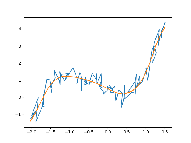
A noisy polynomial being fitted by a neural network.
That’s a pretty nice fit. It totally avoids overfitting, and it doesn’t require any input about the degree of the polynomial (while it is true that the information does exist within the program, the neural net training never accesses it). It is possible if you let it run for an absurd amount of time it would overfit. But because we’re limiting it to a reasonable amount of time, it should produce nice, smooth fits.
Another nice thing about this program is that it updates live after every generation. You can see this in the output, which should be showing the RSS and printing that it saved the data and current fit to a file. If you open that file (fitted-curve.png), you’ll be able to see the neural net’s output updating in real time, which gives an interesting perspective on the way it fits to data.
Fitting Real Data Sets
Now that we have a working model, let us try applying it to a real-world data set. Any data set used for regression training can be used for this purpose, but the one we will be using is a dataset about used car prices based on a number of factors. The specific influencing factor we will be focusing on, though, is the listing price of the car. While these may seem similar, there can be a significant difference between them, with some cars being marked down by over half. Regardless, it is still easy to see the correlation, and thus it is a good data set to fit. Because of the adaptability we coded into the model, the only thing we have to change is the function that returns the data. Right now it returns a given polynomial with some noise added. We can replace this with a data reading function to extract the data from a .csv file, in this case ‘car_data.csv’. To get this file, you can use:
$ wget https://codeberg.org/imahumanperson/serious-programming-courses/raw/branch/main/small-courses/neural-net-basics/car_data.csv
This dataset is originally from Kaggle, an online dataset sharing website. However, it requires creating an account, so we instead opted to download from a git repository containing a copy of the set.
Now, there are two new functions we need to add. The first is the data extraction, and is fairly straightforward:
def read_data(filepath):
    """reads and extracts data from the given file"""
    xs = [] # car listing
    ys = [] # car selling prices
    with open(filepath) as car_data:
        for line in car_data:
            values = line.split(',')
            if values[1].isdigit():
                xs.append([float(values[3])])
                ys.append([float(values[2])])
    # rescale data by median data point
    xs = (np.array(xs) / np.median(xs)).tolist()
    ys = (np.array(ys) / np.median(ys)).tolist()
    xy_zip = list(zip(xs, ys))
    xy_zip.sort(key=lambda x: x[0][0])
    outliers = []
    for point in xy_zip:
        if point[0][0] > 7.5: # arbitrary cutoff for outliers
            print(f'Outlier found: {point}')
            outliers.append(point)
            continue # don't double count
        if point[1][0] > 7.5:
            print(f'Outlier found: {point}')
            outliers.append(point)
        for outlier in outliers:
            xy_zip.remove(outlier)
    xs, ys = list(zip(*xy_zip))

    return xs, ys
This function simply replaces the generate_polynomial_data
function, as they serve the exact same role. It works by putting the
data into lists, scaling the ys properly, then sorting them by the
xs. In case you don’t know how the zip() function works, it takes
any number of lists that are the same length as input, and outputs a
list of tuples of corresponding items from the input lists. This makes
it really useful for sorting lists in the same way, as we needed to
here. The second function we need is one to cut down on the amount of
data the net has to crunch through:
def generate_batch(inputs, expected_outputs, batch_size):
    """generates a random batch based on the batch size"""
    shuffle_zip = list(zip(inputs, expected_outputs))
    random.shuffle(shuffle_zip)
    inputs, expected_outputs = list(zip(*shuffle_zip))
    batch_inputs = []
    batch_expected_outputs = []
    for i in range(batch_size):
        batch_inputs.append(inputs[i])
        batch_expected_outputs.append(expected_outputs[i])
    batch_zip = list(zip(batch_inputs, batch_expected_outputs))
    batch_zip.sort(key=lambda x: x[0][0])
    batch_inputs, batch_expected_outputs = list(zip(*batch_zip))
    return batch_inputs, batch_expected_outputs
This function will return a random sample of the data set with a
certain number of elements. It will then sort this batch to make sure
that it’s still in the proper order. This is done to make the program
run smoothly and not take too long. With that being said, let us take
a look at this updated program in lis-dataset-fitting:
from helper_functions import *

def main():
    num_children_per_net = 20
    num_survive = 5
    variance = 0.5
    generations = 30
    batch_size = 75
    net_dimensions = [1,5,5,5,1]
    filepath = 'car_data.csv'

    first_parent = generate_blank_net(net_dimensions)
    xs, ys = read_data(filepath)
    next_gen = make_next_gen([first_parent], xs, ys, num_children_per_net, num_survive, variance) # create first generation

    inputs = []
    expected_outputs = []
    for i in range(len(xs)):
        inputs.append(xs[i][0])
        expected_outputs.append(ys[i][0])  # reformat xs and ys for matplotlib

    for i in range(generations):
        next_gen = make_next_gen(next_gen, xs, ys, num_children_per_net, num_survive, variance, batch_size)
        variance *= 0.97
        print(f'The RSS is {eval_total_cost(next_gen[0], xs, ys) * 1000} after generation {i+1}.') # the times 1000 makes the RSSs a reasonable value

        outputs = []
        for i in range(len(xs)):
            outputs.append(calc_all_layers(xs[i], next_gen[0], generate_layer_dict(next_gen[0])))
        plt.clf()
        plt.scatter(inputs, expected_outputs, s=0.1)
        plt.plot(inputs, outputs)
        plt.savefig('real-data-fit.png')
        print('Figure saved to real-data-fit.png')
    plt.show() # show the final fit

def eval_RSS(net_outputs, expected_outputs):
    """gets RSS for a given set of outputs"""
    RSS = 0
    for i in range(len(net_outputs)):
        for j in range(len(net_outputs[i])):
            RSS += ((net_outputs[i][j] - expected_outputs[i][j]) ** 2) / len(net_outputs[i]) # make error independant of output layer size
    RSS /= len(net_outputs) # make error independant of data set size
    return RSS

def eval_total_cost(net, input_layers, expected_output_layers):
    """properply formats inputs to eval_RSS"""
    net_outputs = []
    layer_dict = generate_layer_dict(net)
    for i in range(len(input_layers)):
        net_outputs.append(calc_all_layers(input_layers[i], net, layer_dict))
    cost = eval_RSS(net_outputs, expected_output_layers)
    return cost / len(input_layers)

def make_children(net, variance, num_children):
    """creates a specificied number of tweaked copies of a given net"""
    children = []
    for i in range(num_children):
        child = nx.DiGraph(net)
        for edge in child.edges:
            child.edges[edge]['weight'] += random.random() * variance - variance / 2
        children.append(child)
    return children

def make_next_gen(parents, input_layers, expected_output_layers, num_children_per_net=20, num_survive=1, variance=0.1, batch_size=50):
    """creates many of copies of a net, tweaks them slightly, then picks out the best ones to create the next generation."""
    children = parents.copy() # make sure RSS doesn't go up
    best_children = []
    costs = []
    batch_inputs, batch_expected_outputs = generate_batch(input_layers, expected_output_layers, batch_size)
    for parent in parents:
        loop_children = make_children(parent, variance, num_children_per_net)
        for child in loop_children:
            children.append(child)
    for child in children:
        costs.append(eval_total_cost(child, batch_inputs, batch_expected_outputs))

    for i in range(num_survive):
        best_child_index = costs.index(np.min(costs))
        best_children.append(children[best_child_index])
        children.pop(best_child_index)
        costs.pop(best_child_index)

    return best_children

def read_data(filepath):
    """reads and extracts data from the given file"""
    xs = [] # car listing
    ys = [] # car selling prices
    with open(filepath) as car_data:
        for line in car_data:
            values = line.split(',')
            if values[1].isdigit():
                xs.append([float(values[3])])
                ys.append([float(values[2])])
    # rescale data by median data point
    xs = (np.array(xs) / np.median(xs)).tolist()
    ys = (np.array(ys) / np.median(ys)).tolist()
    xy_zip = list(zip(xs, ys))
    xy_zip.sort(key=lambda x: x[0][0])
    outliers = []
    for point in xy_zip:
        if point[0][0] > 7.5: # arbitrary cutoff for outliers
            print(f'Outlier found: {point}')
            outliers.append(point)
            continue
        if point[1][0] > 7.5:
            print(f'Outlier found: {point}')
            outliers.append(point)
    for outlier in outliers:
        xy_zip.remove(outlier)
    xs, ys = list(zip(*xy_zip))

    return xs, ys

def generate_batch(inputs, expected_outputs, batch_size):
    """generates a random batch based on the batch size"""
    shuffle_zip = list(zip(inputs, expected_outputs))
    random.shuffle(shuffle_zip)
    inputs, expected_outputs = list(zip(*shuffle_zip))
    batch_inputs = []
    batch_expected_outputs = []
    for i in range(batch_size):
        batch_inputs.append(inputs[i])
        batch_expected_outputs.append(expected_outputs[i])
    batch_zip = list(zip(batch_inputs, batch_expected_outputs))
    batch_zip.sort(key=lambda x: x[0][0])
    batch_inputs, batch_expected_outputs = list(zip(*batch_zip))
    return batch_inputs, batch_expected_outputs

main()
One thing to notice is that in make_next_gen(), there is an extra
line that gets a randomized batch for each generation. This
significantly cuts down on runtime without hampering accuracy too
much. It does mean that RSS can go up between generations, because the
sample of the data we are currently looking at may have a worse fit
across all children than the last generation did. This is fine,
because the RSS will still go down on average over time, and we still
include the parents in the children to make sure that the net cannot
get actively worse overall.
When you run this, you will likely need to change some of the
parameters at the top of main(). Turning down batch_size,
num_children_per_net, num_survive, or generations will all
help make the program run faster. Unless you have an extremely
powerful computer, this will take around 10-15 minutes to run, which
could be a waste of time. Turning batch_size down to 25 or
generations down to 50 would both help significantly reduce total
runtime. Now, let us see the results of this in fig-fitted-data:
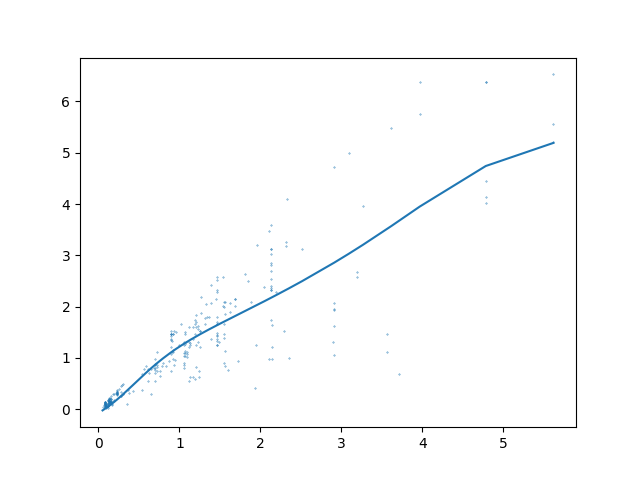
An fitted graph of price vs listing price.
Looking at this graph, there are a couple clear trends. First, most cars tended to be listed low and sell low. While we have rescaled the graph to better suit the needs of the net, you can see the clear clustering around 0, 0. The next trend is that there are basically no data points above y = x. This is because it is very rare for a used car to be haggled up in price, and far more common to be haggled down. There are exceptions; for example, there is a point towards the top right that is above the line. However, this is literally 1 in 2500, and the trend still is very noticeable. Finally, the fitted line is significantly less steep than the y = x points. This shows just how much cars tend to haggled down, usually (based on the slope of the line) 15 - 20%. We have excluded some outliers in this data, namely those that are 7.5x higher than the median of the data in either axis. This is mainly to make the graph easier to read, because the outliers skewed all the other data to the bottom left. In this case, there were only two outliers, so it had very little impact of the quality of the data.
Conclusion
This has been a long and (hopefully) informative chapter, filled with dense terminology and difficult concepts. We started off by understanding what a neural net is, and the basic way it works. In this stage, we visualized example nets with NetworkX and matplotlib. Next, we used a genetic algorithm to fit a neural net to polynomial data. This worked incredibly well, and we got some very smooth and not-overfitted curves.
After that success, we used the same algorithm on a real-world data set: namely, used car price data. The net fit this data quite well, and it showed just how much the average used car will get haggled down. Overall, there are certainly better ways to fit data like this. However, the goal for this chapter was to give a better understanding of neural networks, the genetic algorithm, and RSS, as well as where their strengths and weaknesses lie. Hopefully it does achieve that goal, and you walk away with a new understanding of all of those things.
The methods we used can be applied to more complex problems, and hopefully have endowed you with a greater understanding of the A.I. that has come to be a growing part of our lives. This was only part one of the neural net chapters, and the next one will cover a more advanced algorithm, backpropagation. If you found this interesting I would recommend taking a look at that one as well.