16. Differential Equations
Section author: Sophia Mulholland <smulholland505gmail.com>
16.1. Motivation, Prerequisites, Plan
The goal of this chapter is to learn about differential equations and how they are used to solve scientific problems. We will also learn to write programs in C to solve differential equations.
Differential equations are used to answer scientific questions about how systems change. We will look in to these examples:
A very loose definition of the uses of differential equations is to describe how things change.
how springs move
how populations grow
how radioactive material decays
how bridges collapse
The plan is to start out with a simple explanation of derivatives, and see examples of derivatives in action. We’ll look into the derivation of a falling object’s equation and then Euler’s method. Then we’ll end up modeling a falling body and an oscillating spring.
We give more examples of differential equations in the Ecology chapter.
16.2. Derivatives
If you search for the word ‘derivative’ you’ll find a definition that sounds like this:
- derivative
An expression representing the rate of change of a function with respect to an independent variable.
So the rate of change of a function can change right? It could be going up then down and then up again. So how can we represent the rate of change if it’s not just a number? We use an expression. Like \(2x\) or \(5x^3\). We can use a function to model the rate of change of another function.
Here’s an example of taking a derivative:
There are many different techniques to solve these equations like the Chain rule, the Quotient rule, and the Product rule.
You can graph the functions in gnuplot like this
$ gnuplot
# and at the gnuplot> prompt:
set grid
plot 5*x*x*x-3*x*x+10*x-5
plot 15*x*x-6*x+10
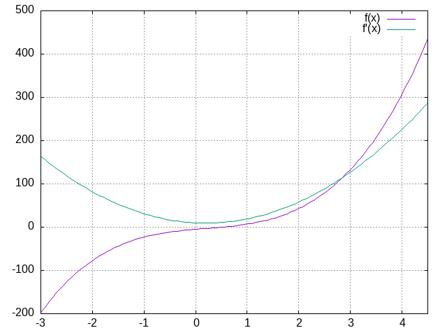
Figure 16.2.1 A function and its derivative. Look at it until you are convinced that the derivative function represents the slope of the original function.
16.2.1. Why?
So why do we care about the rate of change of a function? It helps us predict what’s going to come next. We can predict the future population of earth by analyzing its rate of change right now and making an estimate. We can predict how radioactive material is going to decay.
You can think of a derivative as an instantaneous rate of change.
In the image below, as the two blue points get closer together, we can estimate the slope as the change in \(x\) as it approaches \(0\).
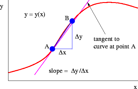
Figure 16.2.2 This photo from the Wikipedia article on derivatives, https://en.wikibooks.org/wiki/Waves/Derivatives shows the concept of taking the derivative
There are real world examples of derivatives all throughout physics, computer science, chemistry, biology, and economics.
Derivatives are an instantaneous rate of change or a slope at one point in time.
16.3. Definitions
- Derivative
An expression representing the rate of change of a function with respect to an independent variable.
- Differential equation
An equation involving a function and one or more of it’s derivatives
- Notations for the derivative:
- \[\begin{split}y'' & = 3x \;\; \textrm{Lagrange notation} \\ f''(x) & = 3x \;\; \textrm{Lagrange notation} \\ \frac{d^2y} {dx^2} & = 3x \;\; \textrm{Leibniz notation} \\ \ddot{y}(t) & = 3t \;\; \textrm{Newton notation (only for functions of time)}\end{split}\]
We have heard lots of talk of equations, and it was probably a reference to algebraic equations, which might look like:
We work out the solutions, possibly by factoring it:
The solution to a system of algebraic equations is a number or set of numbers.
But now we talk about differential equations. An example might look like (in the various notations):
The solution to a differential equation is a function or a family of functions.
16.4. An Example
We know from Newton’s law that
If the force is the force gravity for a falling body, \(F = -mg\), then:
and that
Now
From this, we have proved that the constant \(-g\) is equal to the second derivative of position.
We also know that acceleration is the second derivative of position. How? Well if an object’s position is x, then it’s velocity is the change in x over time.
The acceleration is then the change in velocity over time. \(\frac{dv} {dt}\) or \(\frac{d^2x} {dt^2}\)
16.5. Population Growth
The differential equation describing population growth is:
One way to read this is to think that the more rabbits you have, the more babies you will make in a generation.
How do you solve this? Do you remember which function had a derivative that was equal to itself?
with a constant multiplier in the exponent:
With all that in hand, we can guess that the solution is: \(P(t) = e^{rt}\): this will solve the differential equation.
But wait, now note that if you multiply \(P(t)\) by a constant \(A\), the equation is still satisfied, since you can simplify away any constant multiple of \(P(t)\) in the equation. This means that the most general solution is:
While a pure mathematician might be happy to simply say that you can have an arbitrary constant, a scientist will naturaly ask what the constant means in the system we are studying. And usually there is a good answer. Take a look at what happens at time \(t = 0\):
So \(A\) is the starting value of the population at time 0. We can call it \(P_0\) and write:
To summarize our notation in this problem:
\(P(t)\) is the population at time t
\(P_0\) is the initial population
and \(r\) is the growth rate
Note
This solution is a family of functions, parametrized by the initial population value \(P_0\). Start get used to thinking about differential equations as having families of solutions.
This combination of a differential equation and an initial condition is called an initial value problem. This is very often how we frame problems in physics and other fields (in this case of population growth the field is ecology).
Let’s try to graph a rabbit population with an initial population of 2 rabbits and a growth rate of 0.5:
\(P = 2e^{0.5t}\) is the function
\(\frac{dP} {dt} = e^{0.5t}\) is the function’s derivative
gnuplot
# and at the gnuplot> prompt:
plot 2*exp(0.5*x)
replot exp(0.5*x)

Figure 16.5.1 The growth of the population is in purple and the derivative of that line is in green. Note that as the slope of the rabbit population gets steeper, the derivative also increases.
16.5.1. But what does the derivative tell us?
Since the derivative is positive, the function is increasing.
Since the derivative is increasing, the slope of the function is increasing.
16.6. Euler’s Method
Euler’s Method is a way of approximating the solution of a first-order differential equation. Remember that the solution of a differential equation is always a function or set of functions. To use this method, we need to know the first point on the section we want to look at.
When we don’t know the solution to a particular equation, we can use Euler’s Method. By taking little steps along the graph, it shows us a prediction of what the exact solution looks like.

Figure 16.6.1 From Wikipedia, https://en.wikipedia.org/wiki/Euler_method A picture of the Euler method. The unknown curve is blue, and the approximation is in red.
The idea is that if you have the differential equation and one starting point, you can approximate the solution of the equation. In the figure above, the red line is obviously not curvy like the blue, but why?
At the first point, we have the derivative at a point \((x_1, y_1)\). That means we have the slope at that exact point. We use the slope to graph a tangent line across a time step, which is why they appear to be segments. Then, we have the next two points (hopefully they are close to the actual solution). We calculate the derivative for \((x_2, y_2)\) and repeat the process.
Let’s graph \(y' = 2x - 2\) and use euler’s method to graph its solution \(y = x^2 - 2x\).
It’s much easier to know if we’re right, if we already know the solution. For most differential equations, it is really hard or impossible to solve it analytically.
16.7. Compiling and running C programs
A quick aside to show you how we compile C programs if you have not done this before:
/* a simple "hello world" program in C
   You can compile this with: gcc hello.c -o hello
   and run it with: ./hello
*/

#include <stdio.h>

int main()
{
  printf("hello world\n");
  return 0;
}
You can compile it and run it with:
$ gcc hello.c -o hello -lm
$ ./hello
16.8. A program to use Euler’s method
// this program uses Euler's method to approximate solutions to the
// differential equation dy/dx = f(x, y)

// compile with: gcc euler-method.c -o euler-method -lm
// run with: ./euler-method > euler-method.dat
// plot in gnuplot with:
// plot "euler-method.dat" using 1:2 with lines
// replot  "euler-method.dat" using 1:3 with lines

#include <stdio.h>
#include <math.h>
#include <stdlib.h>

/* prototypes for functions below */
double RHS_parab(double x, double y);
double exact_parab(double x, double y);


int main(int argc, char *argv[])
{
  double xinitial = -5;
  double yinitial = 35;
  double interval = 10; 	/* how many seconds */

  /* handle command line options that allow the user to select number
     of steps */
  int n_steps;
  if (argc == 1) {
    n_steps = 1000;
  } else if (argc == 2) {
    n_steps = atoi(argv[1]);
  } else {
    fprintf(stderr, "error: usage is %s [n_steps]\n", argv[0]);
    return 1;
  }

  /* put out a wee bit of metadata with the "low effort metadata"
     (LEM) structured comment approach */
  printf("##COMMENT: Euler method solution to dy/dx = f(x, y)\n");
  printf("##N_STEPS: %d\n", n_steps);
  printf("##COLUMN_DESCRIPTIONS: x    y_approx    y_exact   slope\n");

  double dx = interval/n_steps;
  double xprev = xinitial;
  double yprev = yinitial;
  double exact = exact_parab(xprev, yprev);
  printf("%lf   %lf   %lf\n", xprev, yprev, exact);
  for (int j = 0; j < n_steps; j++) {
    // calculate right hand side (RHS) with (xi, yi)
    double slope = RHS_parab(xprev, yprev);
    // increase x by step size
    double xnew = xprev + dx;
    // use tangent line to approximate next y value from previous y value
    double ynew = yprev + dx * slope;
    // find exact exact_solution to compare approximation with
    double exact = exact_parab(xnew, ynew);
    printf("%g   %g   %g   %g\n", xnew, ynew, exact, slope);
    // now reset the cycle
    xprev = xnew;
    yprev = ynew;
  }
  return 0;
}

// returns RHS (right hand side)
double RHS_parab(double x, double y)
{
  return 2*x - 2;
}

// returns exact exact_solution
double exact_parab(double x, double y)
{
  return x*x - 2*x;
}
Compile and run and plot this with:
$ gcc euler-method.c -o euler-method -lm
$ ./euler-method > euler-method.dat
$ gnuplot
  # then at the gnuplot> prompt type:
set grid
plot "euler-method.dat" using 1:2 with lines
replot  "euler-method.dat" using 1:4 with lines

Figure 16.8.1 Euler’s approximation with 1000 steps.
At first glance, It looks like the two lines are right on top of each other right? Well if you zoom in on your own graph you can probably see that the lines are not exactly the same. The green line is our exact solution. Using Euler’s method can give us a good approximation for the solution, but it will not be exact.
So now, we can compare that good approximation to a poor approximation using Euler’s method. If you run:
$ ./euler-method 10 > euler-method-bad-approximation.dat
$ gnuplot
  # then at the gnuplot> prompt type:
set grid
plot "euler-method-bad-approximation.dat" using 1:2 with lines title "approximate"
replot  "euler-method-bad-approximation.dat" using 1:4 with linespoints title "exact"

Figure 16.8.2 Euler’s approximation with just 10 steps.
On the purple line there are only ten steps and so it differs a lot from an exact solution of the equation \(\frac{dy} {dx} = 2x - 2\).
16.9. Second Order Differential equations
A second order differential equation is one that involves not just the first derivative of y, but the second one too.
where \(P(x)\) and \(Q(x)\) are continuous functions or constants.
The solutions to second order differential equations will have two arbitrary constants, instead of just one for first order equations. Yes: this is not a coincidence.
Incorporating a second order differential into a real world problem can be really useful. For instance, a model of a ball dropped off a tall building is going to have more than one factor right? To model it’s position, you have to incorporate it’s initial position AND its initial velocity AND it’s acceleration due to gravity.
16.10. Falling Body
Imagine taking a basketball and dropping it off a building. What force is acting on that ball?
Gravity will cause the ball to accelerate towards the ground. So what would we need to model it? The mass of the basketball and the acceleration of gravity.
The way this is described in physics is with Newton’s second law:
We know that for a smallish fall in an ordinary part of the world the force of gravity is \(F = -m g\) (the negative sign is because it is going down), so we end up with this equation:
you can cancel the mass terms to get:
The solution to this equation is one of the simplest cases of indefinite integral applied twice:
where \(C1\) and \(C_2\) are the two arbitrary constants we expect from a second order differential equation. Note that at time \(t = 0\) we can see that
so we can pick better names for the constants: \(v_0\) and \(y_0\) (initial velocity and initial height):
where the physical meaning of the arbitrary constants stands out nicely.
Type in the program below called falling-body.c
// this program uses Euler's method to approximate solutions to the
// falling body equation d^2y/dt^2 = -g

// compile with: gcc falling-body.c -o falling-body -lm
// run with: ./falling-body > falling-body.dat
// plot in gnuplot with:
// plot "falling-body.dat" using 1:2 with lines
// replot  "falling-body.dat" using 1:4 with lines

#include <stdio.h>
#include <math.h>

//acceleration due to gravity
double g = 9.8;
double yinit = 100;
double vinit = 0.1;

double acceleration(double t, double y)
{
  return -g;
}

// returns exact solution
double falling_body_exact(double st)
{
  return yinit + vinit*st - 0.5*g*pow(st,2);
}

int main()
{
  double tinit = 0;

  // define initial variables, step size
  double duration = 10; /* how many seconds */
  int n_steps = 10000;
  double dt = duration/n_steps;

  printf("##COMMENT: Euler method solution to falling body d^y/dx^2 = -g\n");
  printf("##N_STEPS: %d\n", n_steps);
  printf("##COLUMN_DESCRIPTIONS: t    y_approx   v_approx    y_exact   acc\n");

  // set the variables based on our initial values
  double tprev = tinit;
  double yprev = yinit;
  double vprev = vinit;
  double exact = falling_body_exact(tprev);
  double acc = acceleration(tprev, yprev);
  printf("%g   %g   %g   %g   %g\n", tprev, yprev, vprev, exact, acc);
  for (int j = 0; j < n_steps; j++) {
    // solve differential with initial values
    acc = acceleration(tprev, yprev);
    // using acceleration, update velocity
    double vnew = vprev + dt * acc;
    // now, using velocity, update position
    double ynew = yprev + vnew * dt;
    // increase t by step size
    double tnew = tprev + dt;
    tprev = tnew;
    yprev = ynew;
    vprev = vnew;
    // find exact solution to compare approximation with
    double exact = falling_body_exact(tnew);
    printf("%g   %g   %g   %g   %g\n", tnew, ynew, vnew, exact, acc);
  }
  return 0;
}
Compile and run it with:
$ gcc falling-body.c -o falling-body -lm
$ ./falling-body > falling-body.txt
Now use gnuplot to graph the falling body as a function of time
$ gnuplot
  # then at the gnuplot> prompt:
set grid
plot "falling-body.txt" using 1:2 with lines
replot "falling-body.txt" using 1:4 with lines

Figure 16.10.1 Height of a falling body versus time.
16.10.1. Adding Air Resistance to Falling Body
If you consider air drag then the falling body behaves differently. Air drag can often be modeled with an opposing force
where \(b\) is a constant coefficient which depends on the properties of the fluid (in our case air) and the body moving in it.
This drag force gives us this differential equation:
The full solution to this differential equation is possible, though quite gnarly - we discuss the full solution below.
Type or paste in the program below called falling-body-drag.c
// this program uses Euler's method to approximate solutions to the
// falling body equation with air drag: d^2y/dt^2 + g

// compile with: gcc -o falling-body-drag falling-body-drag.c -lm
// run with: ./falling-body-drag > falling-body-drag.dat
// plot in gnuplot with:
// plot "falling-body-drag.dat" using 1:2 with lines
// replot  "falling-body-drag.dat" using 1:4 with lines

#include <stdio.h>
#include <math.h>

//acceleration due to gravity
double mass = 1;                /* kg */
double g = 9.8;                 /* m/s^2 */
double yinit = 100;             /* m */
double vinit = 0.1;             /* m/s */
double b_drag = 0.05;            /*  */

double force(double t, double y, double v)
{
  return -mass*g + b_drag * v * v;
}

// returns exact solution
double falling_body_exact(double st)
{
  return yinit + vinit*st - 0.5*g*pow(st,2);
}

int main()
{
  double tinit = 0;

  // define initial variables, step size
  double duration = 9; /* how many seconds */
  int n_steps = 10000;
  double dt = duration/n_steps;

  printf("##COMMENT: Euler method solution to falling body d^y/dx^2 = -g\n");
  printf("##N_STEPS: %d\n", n_steps);
  printf("##COLUMN_DESCRIPTIONS: t    y_approx   v_approx no_drag_exact acc\n");

  // set the variables based on our initial values
  double tprev = tinit;
  double yprev = yinit;
  double vprev = vinit;
  double exact_nodrag = falling_body_exact(tprev);
  double acc = force(tprev, yprev, vprev) / mass;
  printf("%g   %g   %g   %g   %g\n", tprev, yprev, vprev, exact_nodrag, acc);
  for (int j = 0; j < n_steps; j++) {
    // solve differential with initial values
    acc = force(tprev, yprev, vprev) / mass;
    // using acceleration, update velocity
    double vnew = vprev + dt * acc;
    // now, using velocity, update position
    double ynew = yprev + vnew * dt;
    // increase t by step size
    double tnew = tprev + dt;
    tprev = tnew;
    yprev = ynew;
    vprev = vnew;
    // find exact solution to compare approximation with
    double exact_nodrag = falling_body_exact(tnew);
    printf("%g   %g   %g   %g   %g\n", tnew, ynew, vnew, exact_nodrag, acc);
  }
  return 0;
}
Compile and run it with
$ gcc -o falling-body-drag falling-body-drag.c -lm
$ ./falling-body-drag 1.7 1000 0.4 > falling-body-drag.dat
Now use gnuplot to graph the falling body as a function of time, including drag:
set grid
plot "falling-body-drag.dat" using 1:2 with lines title "with drag"
replot "falling-body-drag.dat" using 1:4 with lines title "without drag"

You will notice that the two plots start out together, but then the plot with drag diverges from the free fall and eventually straightens out.
This straightening out of the slope of \(y(t)\) means that the velocity has become a constant due to air drag balancing out the effects of gravity. This is called the terminal velocity.
To get more insight into what happened you can look at the plots of column 3 (velocity) and column 5 (acceleration). You will see that the velocity starts close to 0, gets very negative very quickly, and then tapers off to about \(-14 m/s\), which is the terminal velocity.
The acceleration, instead, starts at \(-9.8 m/s^2\) and taperes off to zero once the body is moving fast enough that the \(b v^2\) drag force matches the force of gravity.
Now for a discussion of the full solution. There is an article in the Mathematical Poetry blog in which they focus on the question of calculating the velocity.
This they find to be:
The \(\tanh()\) function is integrable, so one can also find \(y(t)\) exactly from this equation, but their main focus is on how to find the terminal velocity:
So the terminal velocity depends on the mass, the acceleration of gravity, and (inversely) on the coefficient \(b\). This matches our intuition, and if we look at the values in our program (at the time of writing this paragraph):
which is what our numerical solution found.
One more thing to say about drag: when certain conditions are satisfied for an object falling in a fluid (or having the fluid move around it), the coefficient \(b\) can be given by:
where \(\rho\) is the fluid density, \(C_d\) is the drag coefficient, and \(A\) is the cross-sectional area of our falling body.
16.11. The harmonic oscillator
The motion of a mass attached to a spring is described by Newton’s law, where the force produced by the spring is given (once you ignore all friction effects) by Hooke’s law:
Here is how to read that equation: \(x\) is a small displacement of the mass when you pull it from its rest position. \(k\) is the sprint constant - a bigger value of \(k\) means that we have a stiffer spring which will return to its resting point more vigorously.
If you push the spring instead of pulling you get (for small displacements) the same force in the opposite direction.
The resulting system is called a “harmonic oscillator”. The Wikipedia page on the harmonic oscillator points out its importance in physics with (approximately) this wording:
The harmonic oscillator model is very important in physics, because any mass subject to a force in stable equilibrium acts as a harmonic oscillator for small vibrations. Harmonic oscillators occur widely in nature and are exploited in many human-made devices, such as clocks and radio circuits. They are the source of virtually all sinusoidal vibrations and waves.
16.11.1. The simple harmonic oscillator
Applying Newton’s law, as we did for the falling body but this time with the spring force, we get:
Let us look at this differential equation in its simplest form. The question that comes to mind is: “what function, when you take its derivative twice, gives you itself back again with a minus sign?”
The answer to that is either \(\sin()\) or \(\cos()\), or an exponential with an imaginary multiple of the argument.
So we expect the solution to look something like:
where \(A\) and \(B\) are the familiar arbitrary constants, and \(C\) is some kind of folding of the parameters of the differential equation, like mass and spring constant.
A harmless simplification is to assume that we are plucking and letting go with an initial velocity of 0, which makes the \(\sin()\) term go away, and we are left with just the cosine term:
If we plug that into the differential equation we see that it works when we set the parameter \(C\) to be:
We usually call this \(\omega_0\), the natural frequency of the oscillator:
and our solution is:
This is a sinusoidal wave with amplitude \(A\) and frequency \(\omega_0\).
The velocity will be:
Think through the proportionalities involved here: the frequency is higher when the spring is stiffer, and lower when the mass is bigger. The same goes for the velocity. Does that match your intuition?
Without any other forces acting on it, this spring will keep going forever.
16.11.2. The damped harmonic oscillator
To model the spring as if it was happening in the real world, we need to account for friction. In physics the force given by sliding friction is usually proportional to the velocity:
adding this to the spring force gives this differential equation for the damped harmonic oscillator:
This can be solved analytically and we get:
If you look at this closely you see that:
The frequency \(omega\) is shifted a bit from the natural \(\omega_0\) of the undamped system. The full relationship is:
\[\omega = \omega_0 \sqrt{1 - \left(\frac{C}{2 \sqrt{m k}}\right)^2}\]There is a damping term \(\exp{(-\zeta \omega_0 t)}\) where \(\zeta = C / (2\sqrt{m k})\). This will make the oscillations damp out very quickly if \(C\) is big, and more gradually if \(C\) is small.
In the program damped-spring-with-friction.c below, you can model
a damped oscillating spring.
// compile with: gcc -o damped-spring-with-friction damped-spring-with-friction.c -lm
// run with: ./damped-spring-with-friction > damped-spring-with-friction.dat
// plot in gnuplot with:
// plot "damped-spring-with-friction.dat" using 1:3 with lines
// replot  "damped-spring-with-friction.dat" using 1:4 with lines

#include <stdio.h>
#include <math.h>

//acceleration due to gravity
double g = 9.8;
//some physics values for the spring equation
double k = 3.0;
double m = 2.0;
//physics for air friction
double air_friction = 3;
//physics for frictional damping force
double damp = 0.5;
/* double damp = 0.0000005; */
double F0 = 10;			/* constant driving force */
double amplitude = 2;

//returns differential
double acceleration(double t, double x, double v)
{
  double omega_0 = sqrt(k / m);
  return - damp * v / m - omega_0*omega_0 * x;
  /* return (-k*x - damp*v + F0*cos(8*t)) / m; */
}

// returns exact solution for harmonic motion
double harmonic_exact(double t)
{
  return amplitude*cos(sqrt(k/m - damp*damp/(4*m*m))*t)*exp((-damp/(2*m)) * t);
}

int main()
{
  double tinit = 0;

  // define initial variables, step size
  double duration = 30; /* how many seconds */
  int n_steps = 10000;
  double dt = duration/n_steps;

  printf("##COMMENT: Euler method solution to damped harmonic oscillator\n");
  printf("###COMMENT: m d^y/dx^2 + C dx/dt + k x = 0");
  printf("##N_STEPS: %d\n", n_steps);
  printf("##COLUMN_DESCRIPTIONS: t    x_approx   v_approx no_damp_exact acc\n");

  // set the variables based on our initial values
  double tprev = tinit;
  double xprev = amplitude;
  double vprev = 0;             /* pluck, then release from rest position */
  double exact_harmonic = harmonic_exact(tinit);
  double acc = acceleration(tprev, xprev, vprev);
  printf("%g   %g   %g   %g   %g\n", tprev, xprev, vprev, exact_harmonic, acc);
  for (int j = 0; j < n_steps; j++) {
    // solve differential with initial values
    acc = acceleration(tprev, xprev, vprev);
    // using acceleration, update velocity
    double vnew = vprev + dt * acc;
    // now, using velocity, update position
    double xnew = xprev + vnew * dt;
    // increase t by step size
    double tnew = tprev + dt;
    tprev = tnew;
    xprev = xnew;
    vprev = vnew;
    // find exact solution to compare approximation with
    double exact_nodamp = harmonic_exact(tnew);
    printf("%g   %g   %g   %g   %g\n", tnew, xnew, vnew, exact_nodamp, acc);
  }
}
Run this program with
$ gcc -o damped-spring-with-friction damped-spring-with-friction.c -lm
$ ./damped-spring-with-friction > damped-spring-with-friction.dat
Now let’s use gnuplot to graph the damped spring:
$ gnuplot
 # and at the gnuplot> prompt:
set grid
set title "damped harmonic oscillator"
set xlabel "time"
set ylabel "amplitude"
plot "damped-spring-with-friction.dat" using 1:2 with lines title  "damped oscillator approximate"
replot  "damped-spring-with-friction.dat" using 1:4 with lines title "damped oscillator exact"
It should look something like this:

If you look at the code you can see that you can do experiments by
changing the damp parameter at the top, and you could even
experiment wtih adding a driving force to the oscillator by changing
the function acceleration().
16.11.3. The non-linear pendulum
The force along the trajectory of mass on a string (pendulum) is:
This gives us an expression of Newton’s law as:
For small angles we have \(\sin(\theta) \approx \theta\), so we get:
this last equation is the same as the simple harmonic oscillator equation, where our fundamental frequency is given by:
once again you should look at the proportionalities in that equation and see if you agree with them.
The full non-linear equation, where we have \(\sin(\theta(t))\), is very difficult to solve. This has been solved in closed form, but the solutions are very complex and involve their own set of approximations to calculate elliptical integrals.
Since the solution is so complex, and the slightest variation in the kind of force we are contemplating would make the equation completely unsolvable, it becomes interesting to use our differential equation solver to calculate it.
Type or paste in the program nonlinear-pendulum.c:
// compile with: gcc -o nonlinear-pendulum nonlinear-pendulum.c -lm
// run with: ./nonlinear-pendulum > nonlinear-pendulum.dat
// plot in gnuplot with:
// plot "nonlinear-pendulum.dat" using 1:3 with lines
// replot  "nonlinear-pendulum.dat" using 1:4 with lines

#include <stdio.h>
#include <math.h>

//acceleration due to gravity
double g = 9.8;
//some physics values for the spring equation
double k = 3.0;
double m = 2.0;
//physics for air friction
double air_friction = 3;
//physics for frictional damping force
double damp = 0.5;
/* double damp = 0.0000005; */
double F0 = 10;			/* constant driving force */
double theta_0 = 0.3;           /* radians */
double Length = 0.5;            /* length in meters */

double acceleration(double t, double x, double v)
{
  return - (g / Length) * sin(x);
  /* return (-k*x - damp*v + F0*cos(8*t)) / m; */
}

// returns exact solution for harmonic motion
double harmonic_exact(double t)
{
  return theta_0*cos(sqrt(g / Length) * t);
}

int main()
{
  double tinit = 0;

  // define initial variables, step size
  double duration = 10; /* how many seconds */
  int n_steps = 10000;
  double dt = duration/n_steps;

  printf("##COMMENT: Euler method solution to damped harmonic oscillator\n");
  printf("###COMMENT: m d^y/dx^2 + C dx/dt + k x = 0");
  printf("##N_STEPS: %d\n", n_steps);
  printf("##COLUMN_DESCRIPTIONS: t    x_approx   v_approx no_damp_exact acc\n");

  // set the variables based on our initial values
  double tprev = tinit;
  double xprev = theta_0;
  double vprev = 0;             /* pluck, then release from rest position */
  double exact_harmonic = harmonic_exact(tinit);
  double acc = acceleration(tprev, xprev, vprev);
  printf("%g   %g   %g   %g   %g\n", tprev, xprev, vprev, exact_harmonic, acc);
  for (int j = 0; j < n_steps; j++) {
    // solve differential with initial values
    acc = acceleration(tprev, xprev, vprev);
    // using acceleration, update velocity
    double vnew = vprev + dt * acc;
    // now, using velocity, update position
    double xnew = xprev + vnew * dt;
    // increase t by step size
    double tnew = tprev + dt;
    tprev = tnew;
    xprev = xnew;
    vprev = vnew;
    // find exact solution to compare approximation with
    double exact_nodamp = harmonic_exact(tnew);
    printf("%g   %g   %g   %g   %g\n", tnew, xnew, vnew, exact_nodamp, acc);
  }
}
Run this program with
$ gcc -o nonlinear-pendulum nonlinear-pendulum.c -lm
$ ./nonlinear-pendulum > nonlinear-pendulum.dat
Now let’s use gnuplot to graph the damped spring:
$ gnuplot
 # and at the gnuplot> prompt:
set grid
set title "damped harmonic oscillator"
set xlabel "time"
set ylabel "amplitude"
plot "nonlinear-pendulum.dat" using 1:2 with lines title  "damped oscillator approximate"
replot  "nonlinear-pendulum.dat" using 1:4 with lines title "damped oscillator exact"
It should look something like this:

Take a careful look at that last plot, and at the source code, specifically the setting of:
double theta_0 = 0.3; /* radians */
0.3 radians is a rather small angle, so the approximation \(\sin(\theta) \approx \theta\) almost holds at \(\sin(0.3) = 0.29552\). But after a few periods you see that the solutions diverge.
If you set theta_0 to be 0.1 then the approximation will work for
a long time. If you set it to be 0.8 you will see the curves diverge
quite soon.