30. Music basics
Areas: acoustics, physics, curiosity
[status: just-starting]
30.1. Motivation, prerequisites, plan
As I write in 2020 we listen to recorded music almost exclusively through a computer. It is interesting, instructive, and useful to understand how the computer represents music, how it is stored, compressed, manipulated, and how interesting things get done with it.
To work through this material you should be comfortable with making
plots, discussed in
Starting out - data files and first plots. You should also install the packages
ffmpeg and sox.
We will start by discussing what sound is. Then we will discuss how it can be represented mathematically. Finally we will look at the various formats that have been devised for computers to store sound files, and how to convert between them.
30.2. What is sound?
Sound is a wave-like sequence of compression and decompression of the air (or other medium). The compression/decompression “front” pushes the next layer of air forward and backwards along the direction of motion. This is called a longitudinal wave.
This can be contrasted with different types of waves, like water waves or electromagnetic waves (light, radio, x-rays, …), where the “up and down” of the wave is perpendicular to the direction in which it moves. Those are called transverse waves.

Figure 30.2.1 Longitudinal waves: the expansion/contraction happens along the direction of motion. (Image from wikipedia.)

Figure 30.2.2 Transverse waves: the expansion/contraction happens perpendicular to the direction of motion. (Image from wikipedia.)
Some gentle introductions to sound can be found at:
https://www.mediacollege.com/audio/01/sound-waves.html
https://www.youtube.com/watch?v=qV4lR9EWGlY
In class we discuss the quantities of interest in talking about sound. Some of these are
amplitude/sound pressure/intensity
frequency/pitch
wavelength
period
speed
pure tone versus superposition of frequencies
30.3. How is sound generated?
Ask the class to discuss various ways in which they have seen sound generated.
Some could be: drum head, guitar soundboard, loudspeaker diaphragm, tweeters, wooferes, …
30.4. Measuring and recording
The human year, before it has been over-exposed to repetitive sounds, can hear from 20 Hz to 20000 Hz (20 kHz).
Microphones usually try to pick up a very clean (non-distorted) signal in the same frequency.
How do microphones work to translate vibration of air into an electrical voltage that changes in time? The lover’s phone, then the carbon microphone, then it gets modern.
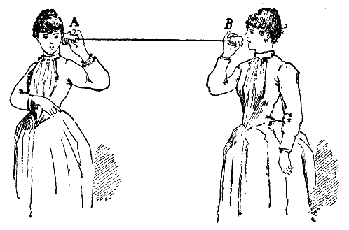
Figure 30.4.1 Robert Hooke’s “Lover’s Telephone”. (Image from wikipedia.)

Figure 30.4.2 A diagram of how the carbon microphon microphone works. When the air compresses it, it conducts more, so you have a higher voltage signal coming out. (Image from wikipedia.)
Can someone research the technical specs of microphones? What is a “frequency response curve”? What would it be for a high quality studio microphone, versus various types of smartphones?
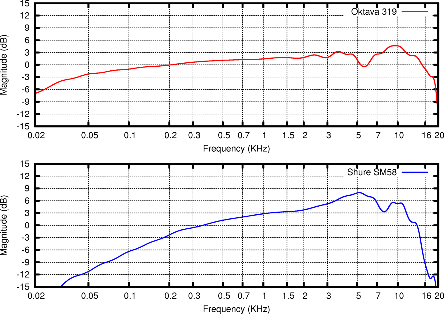
Figure 30.4.3 A “frequency response” curve for two different microphones: the Oktava 319 and the Shure SM58. (Image from wikipedia.)
30.5. What is music
An art form whose medium is sound. Music uses modulations of pitch and amplitude to achieve aesthetical effects.
Discuss some concepts like stereo.
Interesting definitions of “music” proposed by students:
“A sound that is pleasant, has many different …, and doesn’t have to be liked by everyone.”
and
“Many frequencies that move together in a pattern that makes it pleasant to hear.”
30.6. Understanding what we plot in an amplitude plot
Make the following simple plot:
$ gnuplot
 # and at the gnuplot> prompt you can type
plot sin(x)
That shows a basic \(sin()\) wave, but it does not connect to the physical quantities involved. To see how frequency might enter the picture try this out:
$ gnuplot
 # and at the gnuplot> prompt you can type
A = 2.5         # amplitude of 2.5
freq_hz = 440   # 440 hertz - a middle A frequency
set xlabel 'time'
set ylabel 'amplitude'
plot A * sin(2 * pi * freq_hz * x)
This frequency is rather high, so the plot not really showing enough information. To see a bit more you can make the gnuplot sampling higher:
$ gnuplot
 # and at the gnuplot> prompt you can type
set samples 10000
plot A * sin(2 * pi * freq_hz * x)
Clearly we have to zoom in. To show just a few full periods of the wave let us restrict the domain:
$ gnuplot
 # and at the gnuplot> prompt you can type
plot [-0.01:0.01] A * sin(2 * pi * freq_hz * x)
Now we are ready to talk about how to read those axes. Look for the period, understand how the amplitude, frequency, and period appear on it. Discuss why the \(2 \pi\) is in there.
30.7. How does the GNU/Linux microphone work?
We will use the programs rec and play, both of which are part
of the sox package in most distributions.. rec will record a
sound, and play will play it back.
As we saw in the chapter Advanced plotting, you can invoke them like this:
rec myvoice.dat
then speak in to it, or play some music in to it, and hit control-C after just a couple of seconds.
You can play it back with
play myvoice.dat
If you list your directory you will find that the file myvoice.dat has been created, and it has three columns: time, left channel, right channel.
We will plot this file like this:
$ gnuplot
 # and at the gnuplot> prompt you can type
plot 'myvoice.dat' using 1:2 with lines   # you can also try 1:3
30.8. Generating your own musical tone
30.8.1. A single tone
So how would you generate a tone yourself?
#! /usr/bin/env python3

"""Demonstrate generating a pure sin() tone, and printing it out in the sox
simple ascii format.

Run this with
./play_freq.py > tone.dat
and play it to the speaker with
play tone.dat
"""

from math import sin, pi


def main():
    play_freq(2, 200.00, 90000, 4) # play 90000 samples at 48kHz
    play_freq(2, 440.00, 90000, 1) # play 90000 samples at 48kHz
    play_freq(2, 523.25, 40000, 3.0) # play 70000 samples at 48kHz
    play_freq(2, 1000.00, 40000, 0.2) # play 70000 samples at 48kHz
    play_freq(2, 261.63, 40000, 0.6) # play 70000 samples at 48kHz
    # you could duplicate this line with further tones, like with
    # frequency 523.25 Hz

    # you could also play a sequence:
    # freq_sequence = [261.63, 293.66, 329.63, 349.23, 392.00, 440.00, 493.88, 523.25]
    # for freq in freq_sequence:
    #     play_freq(2, freq, 10000)

def play_freq(time, freq, n_samples, amplitude):
    """Plays the note specified by freq, for a duration of n_samples,
    starting at the given time.  Note that if freq is zero then we
    are basically playing a rest note."""
    # 48 kHz seems to be common, and laptop microphones seem to sample
    # at that rate, so let's use it
    sample_rate = 48000
    print('; Sample Rate %d' % sample_rate) # put headers at the top of the file
    print('; Channels 2')

    for i in range(int(n_samples)):
        time = time + 1.0 / 48000.0
        left = amplitude * sin(2*pi*freq*time) # simple sin wave
        right = amplitude * sin(2*pi*freq*time)
        print('%16.10f      %16.10f      %16.10f' % (time, left, right))
    return time

def square_wave(x):
    if x % (2*pi) < pi:
        return 1
    else:
        return -1

main()
Put this into a file with:
$ chmod +x play_freq.py
$ ./play_freq > note.dat
$ play note.dat
The frequencies for “do, re, mi, fa, sol, la, si, do” (C,D,E,F,G,A,B,C) are (in Hertz): 261.63, 293.66, 329.63, 349.23, 392.00, 440.00, 493.88, 523.25.
Note that you could change your main() function to play a full
scale of notes, and it might look like this:
def main():
    play_freq(2, 440.00, 70000)    # play 100000 samples at 48kHz
    play_freq(2, 523.25, 70000)    # play 100000 samples at 48kHz
    # freq_sequence = [261.63, 293.66, 329.63, 349.23, 392.00, 440.00, 493.88, 523.25]
    # for freq in freq_sequence:
    #     play_freq(2, freq, 10000)
30.8.2. From notes to frequencies
Let us take the Italian (Do, Re, Mi, Fa, Sol, La, Si) or German/English (A, B, C, D, E, F, G) notation for musical notes and figure out how to convert those into frequencies. This will allow us to write more versatile programs that take a music specification and play it out.
The general mathematical formula is:
where \(A4_{freq}\) is the frequency of the “A above middle C”
note, 440 Hz. This is discussed in more detail at
https://en.wikipedia.org/wiki/Musical_note#Note_frequency_(hertz)
If we want to convert English
def note2freq(octave, note, sharp_or_flat):
    """Takes a note specification and returns the frequency of that note.
    If note is 'rest' then we return a frequency of zero."""
    ## refer to https://en.wikipedia.org/wiki/Musical_note#Note_frequency_(hertz)
    if note == 'rest':
        freq = 0
    else:
        A4_freq = 440               # A above middle C
        n_steps = note2steps(octave, note, sharp_or_flat)
        freq = A4_freq * math.pow(2, n_steps/12.0)
    return freq
This function relies on another function note2steps() which is too
long to put here, so we will make a link to a full music generating
program generate_music.py which you can study and modify.
You can generate_music.py and save it to a file and play it to
your speaker with:
$ chmod +x generate_music.py
$ ./generate_music.py > popcorn.dat
$ play popcorn.dat
30.9. File formats
The .dat files we have seen are in the simplest possible format. They are not very expressive and they would become huge if we had a long signal. Even those 2-second files were much too big.
We will explore .dat, .au, .aiff, .mp3, .ogg, .webm, .wav, .flac, discussing how each one comes up.
https://en.wikipedia.org/wiki/Timeline_of_audio_formats
30.10. Converting our ascii music .dat files to other formats
Some of the file formats are very well defined: they can be decoded and played by a program that knows the specification for that format. Sometimes there is even an international expert panel which proposes and maintains the specification for that format. There have been oddities associated with this process: due to an oversight by the mp3 standard group, they allowed the mp3 format to involve a patented algorithm, which for a long time made the format unusable by free software. (The patent has expired now.)
The ascii .dat files we have been using here are not one of those
well-specified formats. As far as we can tell, they are only used by
the programs in sox (sound exchange) software swite: rec,
play, and sox.
On the other hand these ascii files are extremely useful for us to
understand them, plot them, and write programs that read and write
them. Our play_freq.py and generate_music.py programs
generate this format with no effort at all.
To convert our output file popcorn.dat (generated in
Section 30.8.2) into the more standard
.flac or .mp3 formats. The sox utility will get us out of the
non-standard .dat format by turning it into a .aif file. From
there we can then use the ffmpeg program to convert it into dozens
of other formats.
For example:
$ ./generate_music.py > popcorn.dat
$ sox popcorn.dat popcorn.aif
$ ffmpeg -i popcorn.aif popcorn.flac
$ ffmpeg -i popcorn.aif popcorn.mp3
$ ls -lsh popcorn.*
Here is the output I get from listing those music files in their various formats:
5.9M -rw-rw-r-- 1 markgalassi markgalassi 5.9M Jan 14 13:26 popcorn.aif
 45M -rw-rw-r-- 1 markgalassi markgalassi  45M Jan 14 13:26 popcorn.dat
1.1M -rw-rw-r-- 1 markgalassi markgalassi 1.1M Jan 14 13:26 popcorn.flac
252K -rw-rw-r-- 1 markgalassi markgalassi 251K Jan 14 13:27 popcorn.mp3
This gives a really interesting look at the effect of using these
various file formats. The original popcorn.dat file is 45
megabytes in size (this should strike you as way too big). Once you
convert to the 1988 vintage audio interchange file format (aif) file
popcorn.aif it is down to about 6 megabytes. The modern free
lossless audio codec (flac) format is 1.1 megabytes, and if you are
willing to lose a small amount of musical quality with the “lossy”
mp3 format you can get it down to a quarter of a megabyte.
You could now play the flac or mp3 file using a music or video program. A quick way from the command line is to run:
$ vlc popcorn.flac