26. Basic agent-based modeling
Section author: Almond Heil <almondheil@gmail.com>
26.1. Motivation, Prerequisites, and Plan
In this chapter, we will learn the basics of agent-based modeling by creating and customizing a simple model using the Mesa framework. While following along, you should keep in mind that the Mesa framework is one of many ways to approach agent-based modeling in Python.
An agent-based model takes a bottom-up approach to solving a problem, by considering the smallest indiviual members (or agents) that make up a larger system and examining how they interact with each other.
Before you start, make sure you fulfill the following prerequisites.
The 10-hour “serious programming” course
This program will have heavy dependencies, so we will use a python virtual environment:
$ sudo apt install python3-venv python3-pip
$ python3 -m venv mesa-venv/
$ source mesa-venv/bin/activate
Installing the required packages with pip.
$ # (now you should have a prompt indicating you are in the vent)
$ pip3 install mesa solara altair
$ pip3 install networkx matplotlib
Now that you’re ready, here’s what we’ll be doing in today’s course!
Learn about the basics of agent-based modeling and object-oriented programming
Create the classes for a simple infection model
Place agents in space and move them
Create a visualization of the model
Manage infection spread among agents
Gather and plot data
26.2. Conceptualizing the model
When building an agent-based model, it’s important to consider the basic building blocks that will make up our model. Based on the broad idea of how diseases spread, we will narrow our focus to how diseases spread by direct contact.
To understand our model as it develops, it’s important to understand a few terms, both from agent-based modeling and object-oriented programming. Some short definitions appear below.
26.2.1. Agent-Based Modeling Concepts
- model
An abstraction of reality seeking to distill the behaviors of a complex system so we can understand it more easily.
In Mesa, the model is specifically the structure that manages setting up and running your program, including the agents inside of it.
- agent
One of the entities within an agent-based model (wow, what a circular definition!) It can interact with other agents and the world in various ways.
- step
A single unit of time in the model. Can also refer to a method an agent follows every time unit.
26.2.2. Object-Oriented Programming Concepts
- class
An object-oriented programming concept which refers to a structure containing the framework for making objects–what they can do, what data they hold, etc.
- object
One instance of a class, which inherets the structure that’s been set up for it. We’ll take advantage of this to create many agent objects based on a single class.
- method
A function that belongs to a class, and can be called by any object based on that class. For instance, we might expect each agent to be able to move around with an
agent.move()method.
26.3. Classes and steps
To implement these concepts, we’ll create a model. Create a file
called direct_contact_step1.py and enter this code.
#! /usr/bin/env python3

from mesa import Agent, Model

class InfectionAgent(Agent):
    def __init__(self, model, infected):
        super().__init__(model)
        self.infected = infected

    def step(self):
        print(f"agent {self.unique_id}; infected {self.infected}")


class InfectionModel(Model):
    def __init__(self, N, seed=None):
        super().__init__(seed=seed)
        self.num_agents = N

        for i in range(self.num_agents):
            # agent number 0 is born infected
            is_infected = True if i == 0 else False
            a = InfectionAgent(self, is_infected)
            self.agents.add(a)

    def step(self):
        self.agents.shuffle_do('step')
Above, we define two classes. InfectionAgent is based on Mesa’s agent
class, and we define how it acts when it initializes and when it
steps. By using super().__init__(model) in the InfectionAgent’s
intialization code, we tell it to set up state common to all agents
(for example, a unique ID). We also set the agent’s infected status to
false, which we’ll edit down the line to start an infection.
InfectionModel is based on Mesa’s model class. When it initializes,
it creates a schedule to run the model with and adds agents to it,
passing them the model parameter.
Now, it’s time to see the code in action! In your terminal, open a
live Python session by typing python3 and enter the following.
>>> from direct_contact_step1 import *
>>> model = InfectionModel(10)
>>> model.step()
You will see the program output something like this.
agent: 1 infection: False
agent: 5 infection: False
agent: 9 infection: False
agent: 8 infection: False
agent: 4 infection: False
agent: 3 infection: False
agent: 7 infection: False
agent: 2 infection: False
agent: 6 infection: False
agent: 0 infection: False
If you repeat model.step(), you will notice that the order the
agents call out is different each time. This is because of the call to
self.agents.shuffle_do('step') in the model’s step() method.
Note
When you want to test changes you’ve made to your model, make sure
to exit your python interpreter with Control+D or by typing
exit(). Then, start a new session and import the code again to
see your most recent changes take effect.
26.4. Space and movement
Now that each agent is able to take steps, we will add space and movement to our model. For this example we will be using a grid for simplicity, as well as Mesa’s built-in support for grid visualization.
To keep everything straight you might want to copy the file
direct_contact_step1.py to a new filename, like
direct_contact_step2.py with:
$ cp direct_contact_step1.py direct_contact_step2.py
and we will edit and make modifications to direct_contac_step2.py
First, we import the necessary components to our project. In this case we want to use a MultiGrid, so that multiple agents can be on top of each other in the same grid cell.
from mesa import Agent, Model
from mesa.space import MultiGrid
Then, we can edit out model’s __init__ method to let it take width and height parameters. We also change our method of placing agents to give them random positions using the model’s random number generator. This generator functions just like the normal Python random module, but it allows us to easily set seeds if we want to reproduce our results down the line.
class InfectionModel(Model):
    def __init__(self, N, width, height, seed=None):
        super().__init__(seed=seed)
        self.num_agents = N
        self.grid = MultiGrid(width, height, torus=True)

        for i in range(self.num_agents):
            # agent number 0 is born infected
            is_infected = True if i == 0 else False
            a = InfectionAgent(self, is_infected)
            x = self.random.randrange(self.grid.width)
            y = self.random.randrange(self.grid.height)
            self.grid.place_agent(a, (x, y))
            self.agents.add(a)
The third argument of MultiGrid represents whether the space is toroidal, meaning that agents who walk of one edge of the grid will reappear on the other side. This emulates an infinite space, and helps us avoid issues with agents hiding in corners or being trapped and unable to move.
To add movement, we need to change what happens when an agent takes a
step. First, add the move() method (maybe just after the
step() method), which tells the agent to move to a random cell
near itself:
def move(self):
    x, y = self.pos
    x_offset = self.random.randint(-1, 1)
    y_offset = self.random.randint(-1, 1)
    new_position = (x + x_offset, y + y_offset)
    self.model.grid.move_agent(self, new_position)
Now we’ve defined how the agent moves, but we have not yet told it to
do that when step() gets called. Go ahead and add the instruction
to move, and also update the print statement to tell us the agent’s
position – right now nothing’s going to show up onscreen.
def step(self):
    self.move()
    print(f"agent {self.unique_id}; pos {self.pos}; infected {self.infected}")
Now, try running the code again–with one difference. Now that the model takes parameters for its width and height, we need to provide those when we create it like so.
>>> from direct_contact_step2 import *
>>> model = InfectionModel(10, 30, 20)
>>> model.step()
If you’re having any issues, go ahead and check your work so far
against this example. You can do so using diff -u in the command
line. Of course, I’m not going to stop you from copy-pasting this
working example, but c’mon.
#!/usr/bin/env python3

from mesa import Agent, Model
from mesa.space import MultiGrid

class InfectionAgent(Agent):
    def __init__(self, model, infected):
        super().__init__(model)
        self.infected = infected

    def move(self):
        x, y = self.pos
        x_offset = self.random.randint(-1, 1)
        y_offset = self.random.randint(-1, 1)
        new_position = (x + x_offset, y + y_offset)
        self.model.grid.move_agent(self, new_position)

    def step(self):
        self.move()
        print(f"agent {self.unique_id}; pos {self.pos}; infected {self.infected}")

class InfectionModel(Model):
    def __init__(self, N, width, height, seed=None):
        super().__init__(seed=seed)
        self.num_agents = N
        self.grid = MultiGrid(width, height, torus=True)

        for i in range(self.num_agents):
            # agent number 0 is born infected
            is_infected = True if i == 0 else False
            a = InfectionAgent(self, is_infected)
            x = self.random.randrange(self.grid.width)
            y = self.random.randrange(self.grid.height)
            self.grid.place_agent(a, (x, y))
            self.agents.add(a)

    def step(self):
        self.agents.shuffle_do('step')
26.5. Visualization
Now we are able to move the agents, but we have no idea of where they are going. Of course, you could add the print statement back in, but with the constant movement and random schedule order it becomes difficult to keep track of what’s going on. To make this easier, we want to add visualization.
Before we make changes let us copy to a new filename, this time from
direct_contact_step2.py to direct_contact_step3.py
$ cp direct_contact_step2.py direct_contact_step3.py
You can right away add this line to the import statements at the top:
from mesa import Agent, Model
from mesa.space import MultiGrid
from mesa.datacollection import DataCollector
Then add a function compute_infected() at the top of
direct_contact_step3.py, just after the import statements and
just before the definition of the classes. This
compute_infected() function will play a role in the visualizations
later on.
# [...]
from mesa.datacollection import DataCollector

def compute_infected(model):
    n_infected = 0
    for agent in model.agents:
        if agent.infected:
             n_infected += 1
    return n_infected

class InfectionAgent(Agent):
    def __init__(self, model, infected):
        # [...]
We then need to add one instruction to our main
direct_contact_step3.py file. In the init method for
InfectionModel, add the line self.running = True and a line to
initialize a “data collector”. It should now match the code below:
def __init__(self, N, width, height, seed=None):
     super().__init__(seed=seed)
     self.num_agents = N
     self.grid = MultiGrid(width, height, torus=True)
     self.running = True
     self.datacollector = DataCollector(
         model_reporters = {"Infected": compute_infected})
Now, we need to create a visualizer which will display our model and
let us interact with it. In this case, we’ll be using Mesa’s built-in
visualization tools because they’re accessible and work well for our
purposes. Create a new file called visualization_step3.py and add
the following to it.
#!/usr/bin/python3

from mesa.visualization import SolaraViz, make_plot_component, make_space_component

# change this to match your file name if it's not direct_contact_step3.py!
from direct_contact_step3 import *

# The parameters we run the model with.
# Feel free to change these!
model_params = {"N": 30,
                "width": 15,
                "height": 10}

def agent_portrayal(agent):
    portrayal = {"Shape": "circle",
                 "color": "grey",
                 "Filled": "true",
                 "Layer": 0,
                 "r": 0.75}
    if agent.infected:
        portrayal["color"] = "LimeGreen"
        portrayal["Layer"] = 1
    return portrayal

infection_model = InfectionModel(model_params["N"],
                                 model_params["width"],
                                 model_params["height"])
SpaceGraph = make_space_component(agent_portrayal)
InfectedPlot = make_plot_component("Infected")

page = SolaraViz(infection_model,
                 model_params=model_params,
                 components=[SpaceGraph, InfectedPlot],
                 name="Infection Agent visualization")

# if you are using a jupyter notebook then you should uncomment this line that
# just says "page"; otherwise you need to run the program with "solara run
# visualization_step3.py"

# page
There’s a lot to unpack in this block of code, because a lot is going
on under the hood with Mesa’s modules. First, we create a dictionary
called params. It holds the names and values for each parameter
the model takes in its __init__. Under the hood, Mesa is unpacking
this dictionary to use the values as keyword arguments or kwargs,
which are used in "name": value pairs to initialize the model.
Next, we define the function agent_portrayal. It takes an
individual agent from the model as input, and returns the necessary
information to draw the agents. Mesa takes care of its visualization
with a web browser window, which handles graphics and user interaction
with JavaScript.
Luckily, we don’t have to deal with the JavaScript side of the equation because Mesa’s SolaraViz module takes care of it - all you will notice is a new tab in your browser pop up. We only need to pass it the portrayal method to use, the dimensions of the grid, and the pixel size of the grid to be displayed.
We then create the infection model, and we also create visual panels
called SpaceGraph and InfectedPlot which you will see when you
run this file.
Finally, we create the visualizer which makes a visualization web page with this line:
page = SolaraViz(infection_model,
                 model_params=model_params,
                 components=[SpaceGraph, InfectedPlot],
                 name="Infection Agent visualization")
This will define the web server. It unites several data structures
we’ve already created. The first term infection_model is the model
to use. The second has the parameters to run the model with. The
third holds a list of the display methods to use (such as the grid we
just defined and the plot of how many are infected). The fourth is
simply the title to display.
See also
The mesa visualization, as of version 3 of mesa, uses the Solara framework to draw graphics into a web browser window. More information is available at: https://solara.dev/
With all this done, we can run the model with a single command from the terminal!
$ solara run visualization_step3.py
Once the server has started it will open a browser window and you can click the “Start” button in the top right to run your model, or the “Step” button move forward incrementaly.
With the server running, you will see a display like this. At this point, you’ll only see the agents wandering around, but we’ll have them spread infection to each other in the next step.
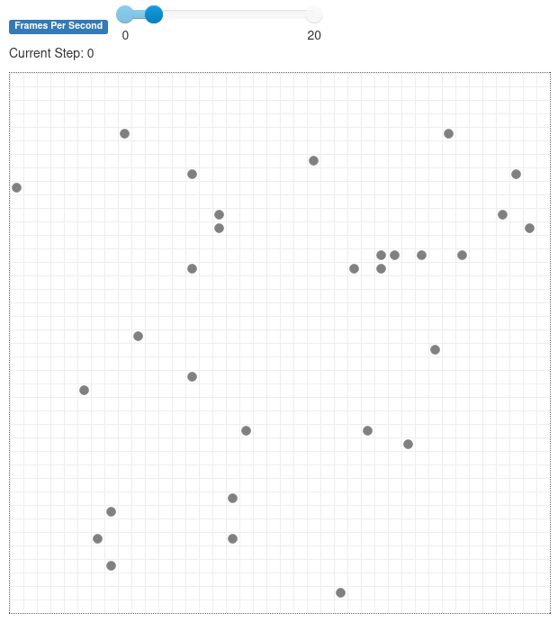
Grid with several grey agents populating it and just one infected green one.
Note
The server won’t automatically quit when you click “Stop” or close the browser tab that is displaying it. To stop the model fully, you have to go to the terminal running the model and press Control+C.
26.6. Interactions between agents
Until now our agents have moved around, and occasionally jostled each other, but they have not yet passed the infection on.
We now add a method for the InfectionAgent class that allows agents to
infect each other. In this method, we use Mesa’s built-in
get_neighbors method to collect a list of all the agents next to a
given point. The parameters “moore” and “include_center” specify what
counts as a neighboring space. Moore means that diagonal spaces are
included, and include_center counts the space that an agent is on.
Start by copying the _step3.py files to _step4.py:
$ cp direct_contact_step3.py direct_contact_step4.py
$ cp visualization_step3.py visualization_step4.py
Quickly edit visualization_step4.py to have:
from direct_contact_step4 import *
But most of our work will be in the direct_contact_step4.py file
where we will adjust the agent model to be infectuous. Start by
adding the method infect_neighbors() to the InfectionAgent class:
def infect_neighbors(self):
    neighbors = self.model.grid.get_neighbors(self.pos, moore=True,
                                              include_center=True)
    for neighbor in neighbors:
        if self.random.random() < 0.25:
            neighbor.infected = True
Next, we’ll edit the agent step method to infect any neighbors only if it is infected.
def step(self):
    self.move()
    if self.infected:
        self.infect_neighbors()
    print(f"agent {self.unique_id}; pos {self.pos}; infected {self.infected}")
As you’ll notice, we take an extremely simple aproach to infection: For each of our direct neighbors, we have a 25% chance of infecting them.
What other ways might this disease spread (for instance, only by touch when we stood on the same grid cell as another person)? How might you change the code to reflect these differences?
To support the visualization in visualization_step4.py you should
introduce a call to datacollector.collect() in the model’s
step() method. This will be called by the visualization system to
get information for making its plots.
collect() call to the step() method def step(self):
self.agents.shuffle_do('step')
self.datacollector.collect(self)
Run it with:
$ solara run visualization_step4.py
When you run the model now, it will look something like this. This screenshot was taken after some 13 steps, and the infection has spread to a bit less than half the population.
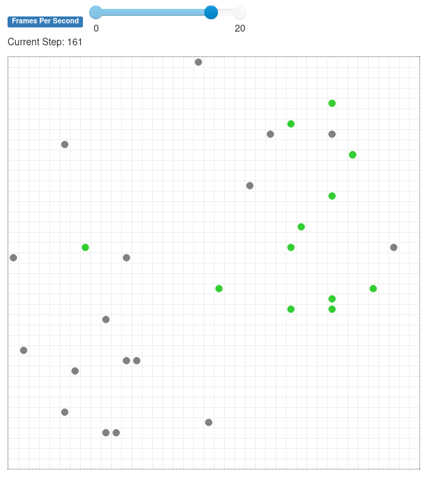
Grid populated with agents, some normal and some infected.
If something isn’t running properly, we give you both programs below:
#! /usr/bin/env python3
from mesa import Agent, Model
from mesa.space import MultiGrid
from mesa.datacollection import DataCollector
def compute_infected(model):
n_infected = 0
for agent in model.agents:
if agent.infected:
n_infected += 1
return n_infected
def infect_neighbors(self):
neighbors = self.model.grid.get_neighbors(self.pos,
moore=True,
include_center=True)
for neighbor in neighbors:
if self.random.random() < 0.25:
neighbor.infected = True
class InfectionAgent(Agent):
def __init__(self, model, infected):
super().__init__(model)
self.infected = infected
def move(self):
x, y = self.pos
x_offset = self.random.randint(-1, 1)
y_offset = self.random.randint(-1, 1)
new_position = (x + x_offset, y + y_offset)
self.model.grid.move_agent(self, new_position)
def infect_neighbors(self):
neighbors = self.model.grid.get_neighbors(self.pos, moore=True,
include_center=True)
for neighbor in neighbors:
if self.random.random() < 0.25:
neighbor.infected = True
def step(self):
self.move()
if self.infected:
infect_neighbors(self)
print(f"agent {self.unique_id}; pos {self.pos}; infected {self.infected}")
class InfectionModel(Model):
def __init__(self, N, width, height, seed=None):
super().__init__(seed=seed)
self.num_agents = N
self.grid = MultiGrid(width, height, torus=True)
self.running = True
self.datacollector = DataCollector(
model_reporters = {"Infected": compute_infected})
for i in range(self.num_agents):
# agent number 0 is born infected
is_infected = True if i == 0 else False
a = InfectionAgent(self, is_infected)
x = self.random.randrange(self.grid.width)
y = self.random.randrange(self.grid.height)
self.grid.place_agent(a, (x, y))
self.agents.add(a)
 def step(self):
     self.agents.shuffle_do('step')
     self.datacollector.collect(self)
#!/usr/bin/python3

from mesa.visualization import SolaraViz, make_plot_component, make_space_component

# change this to match your file name if it's not direct_contact_step3.py!
from direct_contact_step4 import *

# The parameters we run the model with.
# Feel free to change these!
model_params = {"N": 30,
                "width": 15,
                "height": 10}

def agent_portrayal(agent):
    portrayal = {"Shape": "circle",
                 "color": "grey",
                 "Filled": "true",
                 "Layer": 0,
                 "r": 0.75}
    if agent.infected:
        portrayal["color"] = "LimeGreen"
        portrayal["Layer"] = 1
    return portrayal

infection_model = InfectionModel(model_params["N"],
                                 model_params["width"],
                                 model_params["height"])
SpaceGraph = make_space_component(agent_portrayal)
InfectedPlot = make_plot_component("Infected")

page = SolaraViz(infection_model,
                 model_params=model_params,
                 components=[SpaceGraph, InfectedPlot],
                 name="Infection Agent visualization")

# if you are using a jupyter notebook then you should uncomment this line that
# just says "page"; otherwise you need to run the program with "solara run
# visualization_step3.py"

# page
We conclude by showing the final state, in which the entire population has been infected:

Figure 26.8.1 Grid populated with agents, all of them infected.
This simplistic model of infection might be compared to a “zombie apocalypse”: nobody recovers or dies, and eventually the entire population has been infected.
26.7. The final source code
Here are the completed versions of the two final files we produced.
We have removed the _step4 so you can now simply run with:
$ solara run visualization.py
to have the code run and visualize in your browser.
26.8. Making an SIR model
Here are files with a partial implementation of an SIR model based on the simple infection model above.
Download these files:
Remember to run:
$ python3 sir_vis.py
to have the code run and visualize in your browser.
The model seems to work and to show the behaviors you see when you solve the SIR differential equations. After 120 steps we see some oscillation in the S, I, R values:

Figure 26.8.2 SIR model after 120 steps.
And after 360 setps you see a few more oscillations:

SIR model after 360 steps.
26.9. Further reading
You’ve completed this course, but there’s more to look into in this book and elsewhere if you’re interested in agent-based modeling and how agents behave together! Feel free to check out some of the resources below.
The mini-course in Section 27, which covers emergent behavior or how complex behavior emerges from simple rules.
This webpage about SIR and SEIR models for disease. ( Archived at https://web.archive.org/web/20250617163852/https://people.wku.edu/lily.popova.zhuhadar/ ) While it uses equations to describe the trends of disease spread, it is possible to extend the model we made here to create a basic SIR model as well!
The Mesa example boid_flockers, which models bird movement in a flock in continuous space based on Craig Reynolds’ boids
The Wikipedia page and related materials covering Conway’s game of life, an excellent example of emergent behavior.
This journal article going in-depth about modeling the dynamics of disease spread. It’s particularly interesting to see what they decided to model and what they didn’t!
If you feel up to it, see if you can build on the model we made here to make an actual SIR model, where agents only stay infected for a limited amount of time before being removed from the population (or recovered, if you want to put a positive spin on it.)
There are some ordinary differential equations behind SIR models, so based on your mathematical experience you might feel more or less comfortable dealing with them (I’ll admit, they definitely can be scary).
If you’re looking for a place to start, try adding a way for agents to become no longer infected by the disease, and see what questions and problems stem off of that.
You could use the examples above in the files sir_model.py and
sir_vis.py as a starting point.