19. Biology – phylogeny with genetic data

Our simple example with trait data, in the chapter Biology – basics of phylogeny, did not address at all complications that come up when you work with real genetic data.

Caution

From here on, at this time (2026-09-20), we are still forming a coherent set of examples. The links you will find below will be to various DNA sequences, but they are not yet all tested and clear.

19.1. Top level flowchart

A quick mention of the procedure we will follow and the tools we will use:

The sequence of steps for these “real world” examples, in our first rather simple application, will be:

19.2. A simple example of the need for alignment

Let’s talk about this a bit more, since some new jargon is creeping in. Specifically, what’s with sequence alignment and why do we need it?

Start by remembering that in our simple example based on trait data, we had the antelope with sequence:

NYYNY

and the alligator with sequence

NNYYY

Notice something crucial: even though the specific traits were different, their position on the string was always the same! The second trait, for example, was fur. The antelope had Y for fur, while the alligator had N, but at least we knew that we were talking about fur.

Now imagine that we are dealing with real genetic data. When a new species is born, the mutations that lead to its birth might be a simple change of the nucleotide at the same location, or it might involve the insertion or deletion of chunks of the DNA. After all, the evolutionary process is discovering new ways of doing things, which might involve quite a few rearrangements of the DNA layout.

If you have insertion or deletion of pieces of DNA then we have a problem: we cannot compare the two sequences in a “point by point” manner.

Using our traits from before - Features, Fur, Lungs, Gizzard, Jaws - as a hypothetical example, we might ask: “what if we need to distinguish spider monkeys from their close relatives the wooly monkey? One distinguishing trait is that the wooly monkey has thumbs while the spider monkey does not, and relies on its tail for some gripping activities.

Finding information on animal species

The Univerity of Michigan maintains the very useful Animal Diversity Web (ADW). It has entries for the two monkey species we use as examples: Spider Monkeys and Wooly Monkeys.

Our table of traits now could have these headings:

Feathers, Fur, Thumbs, Lungs, Gizzard, Jaws

So if we take our previous table and add this entry we would have our previous data based on the previous table:

>Lamprey
NNNNN
>Antelope
NYYNY
>Sea_Bass
NNNNY
>Bald_Eagle
YNYYY
>Alligator
NNYYY

and now we have two more entries:

>Spider_Monkey
NYNYNY
>Wooly_Monkey
NYYYNY

But wait a second! These new entries have 6 traits with Y(es) or N(no), not 5. So how do we compare them to the others? We will have to insert an extra symbol in the third position for the Lampre, Antelope, Sea Bass, Bald Eagle, and Alligator.

We can take two approaches:

Admit we have a missing trait, but don’t know what to put for it

In this case we might use a star * to denote that ignorance:

>Lamprey
NN*NNN
>Antelope
NY*YNY
>Sea_Bass
NN*NNY
>Bald_Eagle
YN*YYY
>Alligator
NN*YYY
>Spider_Monkey
NYNYNY
>Wooly_Monkey
NYYYNY

Make a statement about the other species having that trait or not

In this case we would say “of those other species, only the eagles have thumbs” and fill out the table like this:

>Lamprey
NNNNNN
>Antelope
NYNYNY
>Sea_Bass
NNNNNY
>Bald_Eagle
YNYYYY
>Alligator
NNNYYY
>Spider_Monkey
NYNYNY
>Wooly_Monkey
NYYYNY

What we have just done is to align the old sequences with the new ones. The result has uniform length.

19.3. Tools for sequence alignment

We will need new tools. First we need to get a the mafft program to realign sequences so they can be compared. We will also need the tools emobss and any2fasta which help with converting file formats.

sudo apt instal mafft
sudo apt install emboss any2fasta

With these tools we can start on a series of examples.

19.4. Example: orchid DNA sequences

More information on some of these examples

The national library of medicine (hosted by the National Institutes of Health, NIH) also stores the publications that went along with the sequencing of certain species. It is interesting, for exampole, to look at the paper that accompanies the California flannelbush (Fremontodendron californicum):

https://pmc.ncbi.nlm.nih.gov/articles/PMC13147169/

which has a link to downlolad the PDF of the paper.

One place to start with more realistic examples is from the biopython-provided example of some 94 orchid species sequences. The example is documented in the bioython library docs

and the file ls_orchid.fasta can be downloaded here:

https://raw.githubusercontent.com/biopython/biopython/refs/heads/master/Doc/examples/ls_orchid.fasta

Remember that it is good to use wget to download data, rather than clicking around in the web browser:

$ wget https://raw.githubusercontent.com/biopython/biopython/refs/heads/master/Doc/examples/ls_orchid.fasta

Let us look at the first two sequences in here and try to glean what is going on in this collection:

>gi|2765658|emb|Z78533.1|CIZ78533 C.irapeanum 5.8S rRNA gene and ITS1 and ITS2 DNA
CGTAACAAGGTTTCCGTAGGTGAACCTGCGGAAGGATCATTGATGAGACCGTGGAATAAACGATCGAGTG
AATCCGGAGGACCGGTGTACTCAGCTCACCGGGGGCATTGCTCCCGTGGTGACCCTGATTTGTTGTTGGG
CCGCCTCGGGAGCGTCCATGGCGGGTTTGAACCTCTAGCCCGGCGCAGTTTGGGCGCCAAGCCATATGAA
AGCATCACCGGCGAATGGCATTGTCTTCCCCAAAACCCGGAGCGGCGGCGTGCTGTCGCGTGCCCAATGA
ATTTTGATGACTCTCGCAAACGGGAATCTTGGCTCTTTGCATCGGATGGAAGGACGCAGCGAAATGCGAT
AAGTGGTGTGAATTGCAAGATCCCGTGAACCATCGAGTCTTTTGAACGCAAGTTGCGCCCGAGGCCATCA
GGCTAAGGGCACGCCTGCTTGGGCGTCGCGCTTCGTCTCTCTCCTGCCAATGCTTGCCCGGCATACAGCC
AGGCCGGCGTGGTGCGGATGTGAAAGATTGGCCCCTTGTGCCTAGGTGCGGCGGGTCCAAGAGCTGGTGT
TTTGATGGCCCGGAACCCGGCAAGAGGTGGACGGATGCTGGCAGCAGCTGCCGTGCGAATCCCCCATGTT
GTCGTGCTTGTCGGACAGGCAGGAGAACCCTTCCGAACCCCAATGGAGGGCGGTTGACCGCCATTCGGAT
GTGACCCCAGGTCAGGCGGGGGCACCCGCTGAGTTTACGC

>gi|2765657|emb|Z78532.1|CCZ78532 C.californicum 5.8S rRNA gene and ITS1 and ITS2 DNA
CGTAACAAGGTTTCCGTAGGTGAACCTGCGGAAGGATCATTGTTGAGACAACAGAATATATGATCGAGTG
AATCTGGAGGACCTGTGGTAACTCAGCTCGTCGTGGCACTGCTTTTGTCGTGACCCTGCTTTGTTGTTGG
GCCTCCTCAAGAGCTTTCATGGCAGGTTTGAACTTTAGTACGGTGCAGTTTGCGCCAAGTCATATAAAGC
ATCACTGATGAATGACATTATTGTCAGAAAAAATCAGAGGGGCAGTATGCTACTGAGCATGCCAGTGAAT
TTTTATGACTCTCGCAACGGATATCTTGGCTCTAACATCGATGAAGAACGCAGCTAAATGCGATAAGTGG
TGTGAATTGCAGAATCCCGTGAACCATCGAGTCTTTGAACGCAAGTTGCGCTCGAGGCCATCAGGCTAAG
GGCACGCCTGCCTGGGCGTCGTGTGTTGCGTCTCTCCTACCAATGCTTGCTTGGCATATCGCTAAGCTGG
CATTATACGGATGTGAATGATTGGCCCCTTGTGCCTAGGTGCGGTGGGTCTAAGGATTGTTGCTTTGATG
GGTAGGAATGTGGCACGAGGTGGAGAATGCTAACAGTCATAAGGCTGCTATTTGAATCCCCCATGTTGTT
GTATTTTTTCGAACCTACACAAGAACCTAATTGAACCCCAATGGAGCTAAAATAACCATTGGGCAGTTGA
TTTCCATTCAGATGCGACCCCAGGTCAGGCGGGGCCACCCGCTGAGTTGAGGC

As a newcomer to this kind of data file I notice a few things:

• The format seems to have a few metadata parts, like the |gi|2765658| and |gi|2765657| strings. These might indicate a unique ID for the alignment. Looking closely at the details of the file format we see that the FASTA format does not specify it very uniformly, but |gi|2765658| is indeed some kind of unique ID.

• Maybe the first species is called C.irapeanum and the second one is called C.californicum.

• The sequences are made of the letters A, G, C, T, so we can deduce that it is a DNA sequence, since those are the letters for Adenine, Thymine, Cytosine, and Guanine.

• They have different lengths!! Clearly these different species of orchids have different length sequences. This means that we will not be able to run a phylogentic analysis program on them directly.

The first tool we will use is mafft. You can realign these sequences with:

$ mafft --auto ls_orchid.fasta > ls_orchid_realigned.fasta

You should now examine these two files visually. The first entry in the realigned (C.irapeanum) file is:

>gi|2765658|emb|Z78533.1|CIZ78533 C.irapeanum 5.8S rRNA gene and ITS1 and ITS2 DNA
cgtaacaaggtttccgtaggtgaacctgcggaaggatcattgatgagaccgtggaataaa
cgatcgagtgaatccggaggaccggtg--tactcagctcaccgggggcatt-gctcccgt
ggtgacc-ctg-atttg-ttgt----tgggccgcctcgggagcgtccatggcgg---gtt
tg-aacctc-tagcccggcgcagtttgggcgccaagccata-------------------
---------------------------------------------tgaaagcatcaccgg
cgaatggcattgt-cttcc--c--caaaa---c--ccggag-cggcggc-gtg-ctgtcg
-c-------------------------g-tgcccaatga-----atttt---ga-tgact
ctc-gc---aaa-c-gggaatcttggctcttt-gcatc-gga-tggaa-gga-cgcagcg
-aaa-tgcgataag-tggtgtgaattgcaagatcccgtgaa-ccatcgagtctttt-gaa
cgcaagttgcgcccgaggccatcaggctaagggcacgcctgcttgggcgtcgcgcttcgt
c--tctctcct---gccaatgcttgcccggc--ata-cagccaggccggcgtggtgcgga
tgtgaaagattggccccttgtgcctaggtgcggcgggtccaagagc----tggtgttttg
atggc-ccggaaccc-ggcaagaggtggacggatgctggcagc-------agc---tgcc
gtgcgaatcccccatgttgtcgtg-cttgtcggacaggcagg------agaacccttccg
aa-ccccaatgga---------------------gggcggttga-ccg-ccattc-gga-
tgtgaccccaggtcaggcgggggcacccgctgagtttacgc

Here are some things you conclude if you look at the complete original and realined files:

ls_orchid.fasta

The original file had some 740 to 941 nucleotides in its sequences. Each sequence could have a different length.

ls_orchid_realigned.fasta

Each sequence now has the same length. Various sub-sequences of nucleotides have been moved around, and in some places sequences of dashes ------ have been inserted. This allows us to compare “apples to apples” in a certain sense: the gene subsequences that exist that don’t exist in a certain spcies are marked as ------ and not compared in calculating genetic differences.

19.5. BELOW HERE NOT YET REVISED

19.6. Example: the plague - Y.pestis

Or try Y.pestis from genbank. Check this page: https://www.ncbi.nlm.nih.gov/nuccore/NC_005816.1 and download with:

$ wget --output-file Y.pestis.gb 'https://www.ncbi.nlm.nih.gov/sviewer/viewer.cgi?tool=portal&save=file&log$=seqview&db=nuccore&report=genbank&id=45478711&&ncbi_phid=CE89312FA824C6B1000000000091008E'

or from reddit https://www.reddit.com/r/bioinformatics/comments/5h4qnc/what_is_the_best_way_to_download_genbank_data/

Saccharomyces cerevisiae
https://en.wikipedia.org/wiki/Accession_number_(bioinformatics)
locus=CP011547
curl -s  "https://eutils.ncbi.nlm.nih.gov/entrez/eutils/efetch.fcgi?db=nucleotide&id=${locus}&rettype=gb&retmode=txt" > ${locus}.gbk

for great whale shark:

locus=JAHMAH000000000

for Y.pestis: locus=CP160598.1

https://www.ncbi.nlm.nih.gov/datasets/taxonomy/7801/

https://www.ncbi.nlm.nih.gov/datasets/genome/?taxon=259920

Note

If our files are in genbank format then mafft (the alignment program) does not work onm that natively. You can convert a collection of .gbk files to a .fasta file with:

sudo apt install emboss any2fasta
for gbk_fname in *.gbk
do
    any2gbk $gbk_fname > ${gbk_fname}.fasta
done

Look at the .fasta files - they have very different sequence lengths, since you have sharks and orchids and plague bacteria. You can use mafft to realign them:

$ cat *.gbk.fasta > multi_species.fasta
$ mafft --auto multi_species.fasta > multi_species_realigned.fasta

Now that we have a basic example out of the way, we are going to try a real-world example. This example is on variations a gene called CRAB across species, and can be copy-and-pasted from this link.

Listing 19.1 a larger fasta format file.

>crab_anapl ALPHA CRYSTALLIN B CHAIN (ALPHA(B)-CRYSTALLIN).             
MDITIHNPLIRRPLFSWLAPSRIFDQIFGEHLQESELLPASPSLSPFLMR
SPIFRMPSWLETGLSEMRLEKDKFSVNLDVKHFSPEELKVKVLGDMVEIH
GKHEERQDEHGFIAREFNRKYRIPADVDPLTITSSLSLDGVLTVSAPRKQ
SDVPERSIPITREEKPAIAGAQRK
>crab_bovin ALPHA CRYSTALLIN B CHAIN (ALPHA(B)-CRYSTALLIN).             
MDIAIHHPWIRRPFFPFHSPSRLFDQFFGEHLLESDLFPASTSLSPFYLR
PPSFLRAPSWIDTGLSEMRLEKDRFSVNLDVKHFSPEELKVKVLGDVIEV
HGKHEERQDEHGFISREFHRKYRIPADVDPLAITSSLSSDGVLTVNGPRK
QASGPERTIPITREEKPAVTAAPKK
>crab_chick ALPHA CRYSTALLIN B CHAIN (ALPHA(B)-CRYSTALLIN).             
MDITIHNPLVRRPLFSWLTPSRIFDQIFGEHLQESELLPTSPSLSPFLMR
SPFFRMPSWLETGLSEMRLEKDKFSVNLDVKHFSPEELKVKVLGDMIEIH
GKHEERQDEHGFIAREFSRKYRIPADVDPLTITSSLSLDGVLTVSAPRKQ
SDVPERSIPITREEKPAIAGSQRK
>crab_human ALPHA CRYSTALLIN B CHAIN (ALPHA(B)-CRYSTALLIN).
MDIAIHHPWIRRPFFPFHSPSRLFDQFFGEHLLESDLFPTSTSLSPFYLR
PPSFLRAPSWFDTGLSEMRLEKDRFSVNLDVKHFSPEELKVKVLGDVIEV
HGKHEERQDEHGFISREFHRKYRIPADVDPLTITSSLSSDGVLTVNGPRK
QVSGPERTIPITREEKPAVTAAPKK
>crab_mesau ALPHA CRYSTALLIN B CHAIN (ALPHA(B)-CRYSTALLIN).             
MDIAIHHPWIRRPFFPFHSPSRLFDQFFGEHLLESDLFSTATSLSPFYLR
PPSFLRAPSWIDTGLSEMRMEKDRFSVNLDVKHFSPEELKVKVLGDVVEV
HGKHEERQDEHGFISREFHRKYRIPADVDPLTITSSLSSDGVLTVNGPRK
QASGPERTIPITREEKPAVTAAPKK
>crab_mouse ALPHA CRYSTALLIN B CHAIN (ALPHA(B)-CRYSTALLIN) (P23).       
MDIAIHHPWIRRPFFPFHSPSRLFDQFFGEHLLESDLFSTATSLSPFYLR
PPSFLRAPSWIDTGLSEMRLEKDRFSVNLDVKHFSPEELKVKVLGDVIEV
HGKHEERQDEHGFISREFHRKYRIPADVDPLAITSSLSSDGVLTVNGPRK
QVSGPERTIPITREEKPAVAAAPKK
>crab_rabit ALPHA CRYSTALLIN B CHAIN (ALPHA(B)-CRYSTALLIN).             
MDIAIHHPWIRRPFFPFHSPSRLFDQFFGEHLLESDLFPTSTSLSPFYLR
PPSFLRAPSWIDTGLSEMRLEKDRFSVNLDVKHFSPEELKVKVLGDVIEV
HGKHEERQDEHGFISREFHRKYRIPADVDPLTITSSLSSDGVLTVNGPRK
QAPGPERTIPITREEKPAVTAAPKK
>crab_rat ALPHA CRYSTALLIN B CHAIN (ALPHA(B)-CRYSTALLIN).             
MDIAIHHPWIRRPFFPFHSPSRLFDQFFGEHLLESDLFSTATSLSPFYLR
PPSFLRAPSWIDTGLSEMRMEKDRFSVNLDVKHFSPEELKVKVLGDVIEV
HGKHEERQDEHGFISREFHRKYRIPADVDPLTITSSLSSDGVLTVNGPRK
QASGPERTIPITREEKPAVTAAPKK
>crab_squac ALPHA CRYSTALLIN B CHAIN (ALPHA(B)-CRYSTALLIN).             
MDIAIQHPWLRRPLFPSSIFPSRIFDQNFGEHFDPDLFPSFSSMLSPFYW
RMGAPMARMPSWAQTGLSELRLDKDKFAIHLDVKHFTPEELRVKILGDFI
EVQAQHEERQDEHGYVSREFHRKYKVPAGVDPLVITCSLSADGVLTITGP
RKVADVPERSVPISRDEKPAVAGPQQK

Note that you may have to trim the ends of the sequences to match the length; while this may lose some information contained in the sequences, it is small enough where the overall pattern will still show in the plot. We can reuse our tree-inferring program from earlier (make sure to change the file to the CRAB one and remove the line that sets the root), and it should produce something like Figure 19.1:

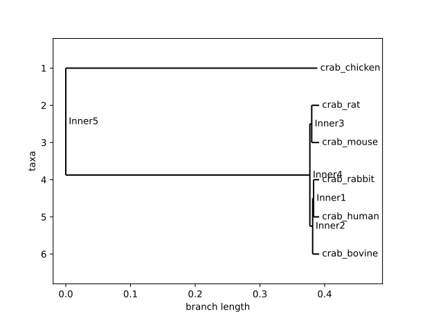
Figure 19.1 A graph showing the differences in the CRAB gene.

This graph shows a trend that makes a lot of sense: the mammals are all closely related, and the chicken is not closely related to them. In addition, the rat and mouse are closely related, which makes sense. The human in most closely related to the rabbit, and then the cow.

Biopython allowed us to learn all that information from meaningless (to us) sequences of letters. This can be incredibly useful for building phylogenetic trees, because you can simply plug in the genomes you are comparing and it will tell you how they are related. It’s not perfect, as we saw, and you may have to define an outgroup to “orient” the program. But other than that, it worked very well, and could build both or specifically engineered tree and a real example of a genome.

This is only a small taste of what biopython can do, and exploring it further would be reqrding for those with an interest in biology. The documentation and examples can be found here.

19.7. Other sequence analysis resources

Berkeley evolution course. 7 organisms and 7 features: https://evolution.berkeley.edu/evolibrary/article/phylogenetics_07

Cute with ladybugs, but just 6 elements and 7 features: https://bioenv.gu.se/digitalAssets/1580/1580956_fyltreeeng.pdf

Another video giving step-by-step for building a tree by hand: https://www.youtube.com/watch?v=09eD4A_HxVQ