8. Fourier analysis on sound and music

When we mentioned waves with different frequencies you might have thought of sound, and you would have been right. Fourier analysis is a good tool for understanding what makes up sound waves.

Let us take a tour through a series of signals, and we will look at their fourier transforms.

Computer programming consideration: we need to run programs to demonstrate this section. But this is not a programming class, and we cannot assume that everyone is running a Linux distribution.

So when I teach the class I demonstrate running of the programs myself, with a brief discussion of what the code is doing and how easy it is to do this. And I also tell the students that those who are have had good advice and are running Linux can download the programs and run them.

To prepare to run all these programs one should first do:

$ sudo apt install gnuplot-qt python3-matplotlib python3-scipy
$ sudo apt install sox ffmpeg

8.1. Tuning fork

A tuning fork puts out a very pure single \(\sin\) wave at a “middle A” note, also known as \(A_{440}\) or \(A_4\) or concert pitch. \(A_4\) has a frequency of 440 Hz.

We can download a stock mp3 file of the sound of a tuning fork, then we can use standard command line utilities to convert it to a text file. For example:

$ wget https://cdn.freesound.org/previews/361/361922_5902584-lq.mp3 -O tuning-fork-440Hz.mp3
$ # convert through various steps to .aif and then to .dat
$ ffmpeg -i tuning-fork-440Hz.mp3 tuning-fork-440Hz.aif
$ sox tuning-fork-440Hz.aif tuning-fork-440Hz.dat
$ ls -lsh tuning-fork-440Hz.*
$ # check out what it sounds like with
$ vlc tuning-fork-440Hz.mp3

(note: another tuning fork, maybe cleaner, is at: https://freesound.org/data/previews/126/126352_2219070-lq.mp3 )

You can plot it with:

$ gnuplot
$  # then at the gnuplot> prompt:
plot 'tuning-fork-440Hz.dat' using 1:2 with lines

This shows you the plot of amplitude versus time, and you should notice some correspondence between it and the sound you heard - the person who recorded this file kept modulating how loud it was.

But that does not tell us what frequencies are in it! Let us adapt the filter_random.py program to work with this data file.

You can download code/fft_audio.py and try running it on this tuning-fork.dat file:

$ python3 fft_audio.py tuning-fork-440Hz.dat

So the bottom line is: once we have it as a text file we can do the following:

Use our standard plotting techniques to see that it looks like a \(\sin\) wave, but with lots of amplitude variation.
Write a program which uses the powerful Python scientific libraries to calculate the Fourier transform of the tuning fork signal.
Look at the Fourier transform, hoping to see that a clean \(\sin\) wave will appear as a single spike, indicating that there is only one \(\sin\) wave in the signal.

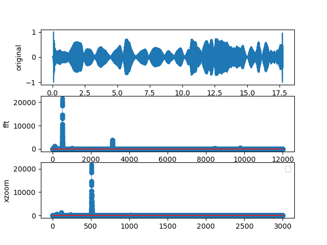
../_images/fft_tuning-fork.png — Figure 8.1.1 The FFT of a tuning fork. Notice the single dominant frequency, which shows that the tuning fork is close to being a perfect \(\sin()\) wave.

8.2. White noise

Now let us download an example of white noise. This is a random wave with no discernible pattern.

$ wget -q --continue http://www.vibrationdata.com/white1.mp3 -O white-noise.mp3
$ ffmpeg -n -i white-noise.mp3 white-noise.aiff
$ sox -q white-noise.aiff -t dat white-noise.dat
$ head -7000 white-noise.dat | tail -2000 > white-noise-small-sample.dat
$ # check out what it sounds like with
$ vlc white-noise.mp3

Notice how we removed some data from the start and some from the end so as to have a shorter data file.

$ gnuplot
$ # then at the gnuplot> prompt:
reset
set grid
plot 'white-noise-small-sample.dat' with lines

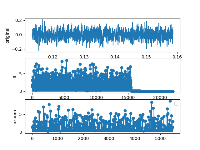
../_images/fft_white-noise-small-sample.png — Figure 8.2.1 The FFT of a white noise sample. Notice the broad and flat value of the transform for almost all the frequencies.

You could say that the Fourier spectrum for white noise is the opposite of that for the pure tuning fork signal: instead of a single spike you have random-looking spikes all over the spectrum.

8.3. Violin playing single “F” note

Now let us look at some musical notes from real instruments. Each note corresponds to a certain frequency, as discussed in [Wikipedia contributors, 2025].

The Fourier transform for this violin note shows a much more complex signal than the tuning fork:

$ wget --continue http://freesound.org/data/previews/153/153595_2626346-lq.mp3 -O violin-F.mp3
$ ffmpeg -n -i violin-F.mp3 violin-F.aiff
$ sox violin-F.aiff -t dat violin-F.dat
$ python3 fft_audio.py violin-F.dat

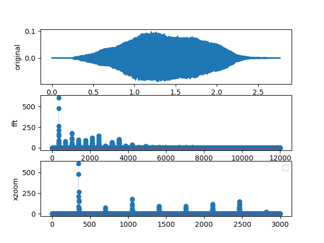
../_images/fft_violin-F.png — Figure 8.3.1 The FFT of a violin play an F note.

The signal in has some structure to it. The Fourier transform has several peaks: the strongest peak (for a \(A_4\) note) will be at the fundamental frequency of 440 Hz, but there are many other peaks. The pattern of the peaks characterizes the sound of that specific violin (or guitar or other instrument).

8.4. Violin playing single “A” note

This is a repeat of but with a different note on the violin: F instead of A. is hard to distinguish from since the character of the instrument is the same. At this point we have not written code to plot the actual frequencies on the \(x\) axis, so we cannot spot that the \(A_4\) note has its highest peak at 440Hz, while the \(F_5\) is at 698.45Hz [Backus, 1977].

$ wget --continue http://freesound.org/data/previews/153/153587_2626346-lq.mp3 -O violin-A-440.mp3
$ ffmpeg -n -i violin-A-440.mp3 violin-A-440.aiff
$ sox violin-A-440.aiff -t dat violin-A-440.dat
$ python3 fft_audio.py violin-A-440.dat

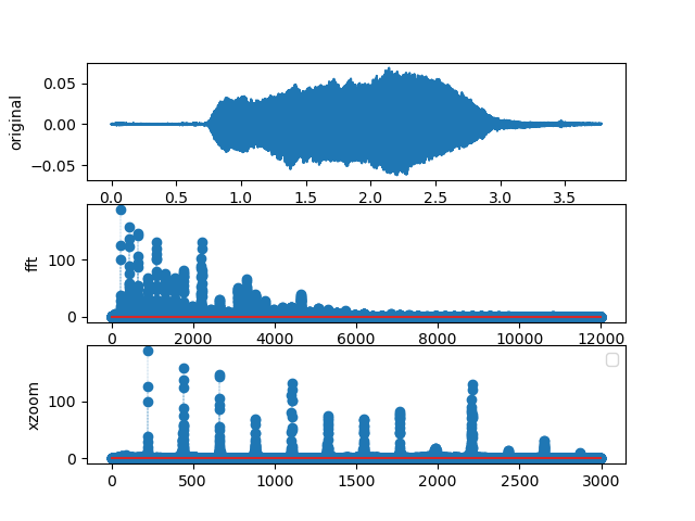
../_images/fft_violin-A-440.png — Figure 8.4.1 The FFT of a violin play a middle A note.

8.5. A more complex music clip

The Pachelbel Canon is a well-known piece of baroque classical music which starts with a single note that is held for a while. shows the signal and its Fourier transform, where you can identify a dominant peak.

$ wget -q --continue http://he3.magnatune.com/music/Voices%20of%20Music/Concerto%20Barocco/21-Pachelbel%20Canon%20In%20D%20Major%20-%20Johann%20Pachelbel%20-%20Canon%20And%20Gigue%20For%20Three%20Violins%20And%20Basso%20Continuo%20In%20D%20Major-Voices%20of%20Music_spoken.mp3 -O Canon.mp3
$ ffmpeg -n -i 'Canon.mp3' Canon.aiff
$ sox -q Canon.aiff -t dat Canon.dat
$ head -50000 Canon.dat | tail -4000 > canon-small-sample.dat
$ python3 fft_audio.py canon-small-sample.dat

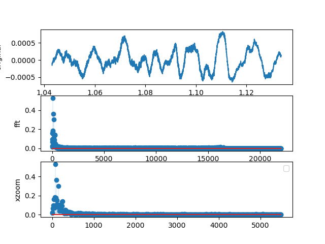
../_images/fft_canon-small-sample.png — Figure 8.5.1 The FFT of the first few seconds of the Pachelbel canon.

But what happens if we have music that is not a single note? In we will look at a clip of a choir singing Gloria in Excelsis Deo. The clip (which you can play with vlc gloria.ogg after downloading it) starts in a place where many voices are singing in harmony, so there is no single note to be picked out.

$ wget -q --continue https://upload.wikimedia.org/wikipedia/en/e/ea/Angels_We_Have_Heard_on_High%2C_sung_by_the_Mormon_Tabernacle_Choir.ogg -O gloria.ogg
$ ffmpeg -n -i gloria.ogg gloria.aiff
$ sox -q gloria.aiff -t dat gloria.dat
$ python3 fft_audio.py gloria.dat

We expect to see several different peaks in the Fourier spectrum, and that is what you see in the second panel of this plot.

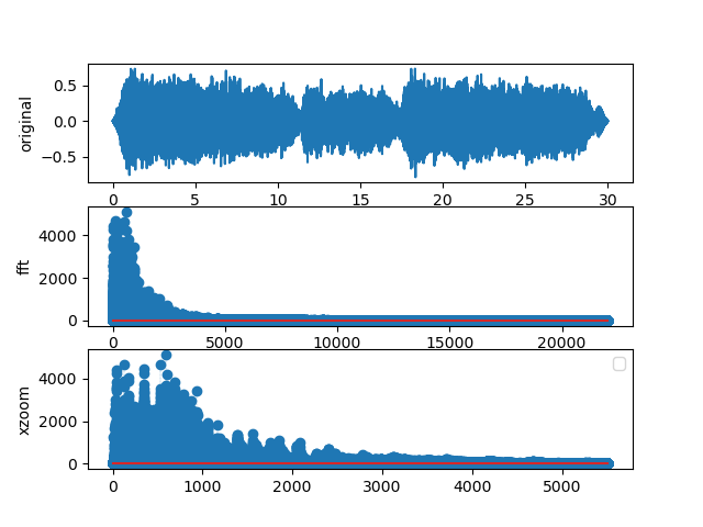
../_images/fft_gloria.png — Figure 8.5.2 The FFT of the first few seconds of Gloria in Excelsis Deo.

8.6. Create your own audio clip and analyze it

Record some sound and analyze it.

The program sox, which we used to do audio format conversion, comes with two other programs rec (to record from your computer’s microphone) and play to play those files back.

To try it out I ran the following:

$ rec mark-guitar-sample.dat
$ ## I played a few guitar notes near the laptop microphone,
$ ## emphasizing low and high frequences, then I hit control-C
$ play mark-guitar-sample.dat
$ python3 fft_audio.py mark-guitar-sample.dat

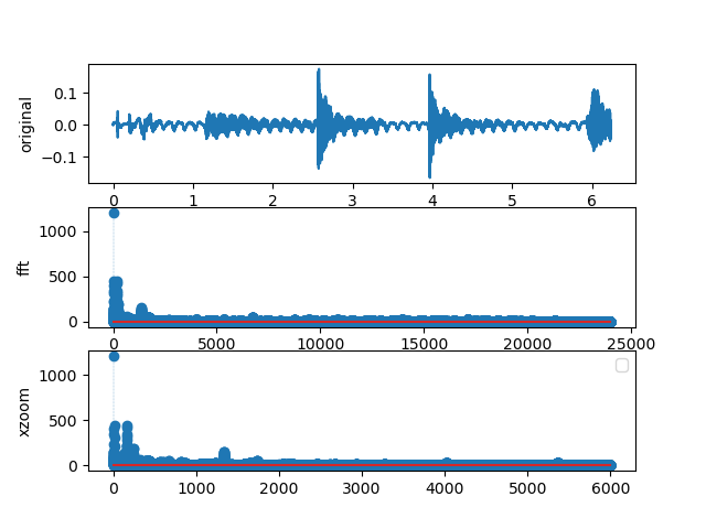
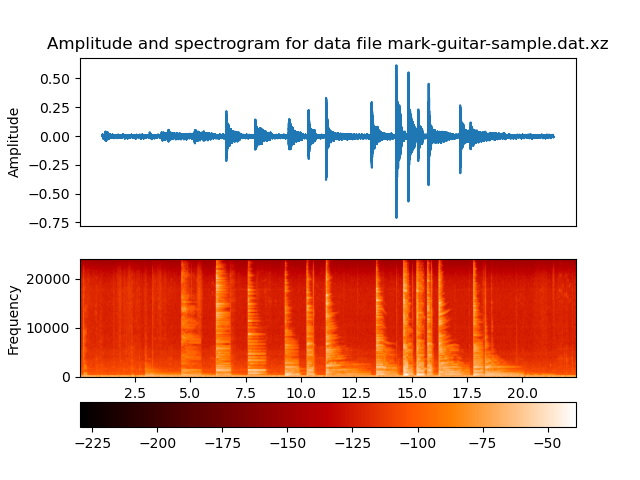
../_images/fft_mark-guitar-sample.png — Figure 8.6.1 The FFT of my own musical sample.

Now try doing this again for different things you can record with your microphone. If you have a tuning fork, tap it and then rest it on a guitar’s soundboard and record that, see if you get something similar to what we saw when we discussed tuning forks. If you have a musical instrument, try recording an A note or an F note and compare them to what we discussed violins.

8.7. A final step: making spectrograms

You can download the program in the mini-courses book:

https://markgalassi.codeberg.page/small-courses-html/plotting-advanced/plotting-advanced.html#id12

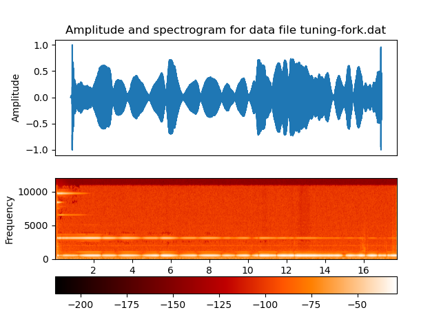
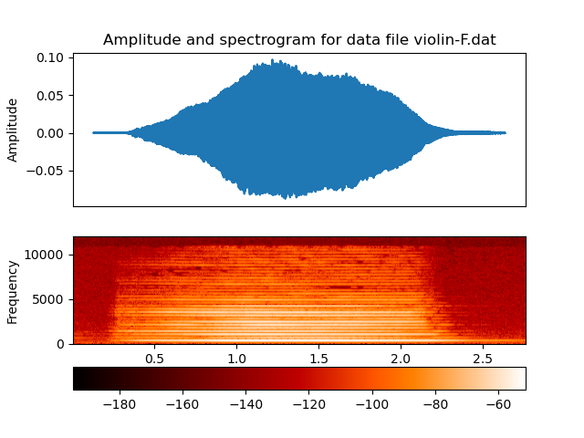
I will show you a set of examples based on the music data files we generated earlier in this chapter:

$ # simple tuning fork
$ python3 music2spectrogram.py tuning-fork.dat