17. Monte Carlo methods

Monte Carlo methods are calculation and modeling techniques in which we use random number sequences to approximate calculations that would be much too difficult otherwise. The name is inspired by the city of Monte Carlo which has a famous casino, which relates to randomness.

There are many areas in which monte carlo methods are the best choice, and we will examine a couple of these.

17.1. Areas, volumes, hypervolumes

17.1.1. Two-dimensions: calculating \(\pi\): with the monte carlo method

This is a good first introduction to monte carlo integration, which allows us to discuss monte carlo methods in general.

The method involves shooting darts into a square which has a circle inscribed in it. Draw the picture of a circle inside a square, and draw points of random darts hitting it.

The fraction of darts that fall in the circle is proportional to the fraction of areas:

\[\frac{N_{\rm cir}}{N_{\rm sq}} \approx \frac{A_{\rm cir}}{A_{\rm sq}}\]

The area of the circle is \(\pi r^2\), and that of the square is \(\pi l^2\). Since we have constructed this so that \(l = 2r\) we get:

\[\frac{N_{\rm cir}}{N_{\rm sq}} \approx \frac{\pi r^2}{(2r)^2} = \frac{\pi}{4}\]

This gives us:

\[\pi = 4 \frac{N_{\rm cir}}{N_{\rm sq}}\]

Now what I usually do is write a live program which has a loop that throws 1000 darts. It does so by calculating x = random.random() * 2 - 1 and the same for y. This gives us a dart in a square. Then using the pythagoras theorm with if sqrt(x*x + y*y) < 1 we can determine if the dart is in the circle. We add all that up and estimate \(\pi\).

Here is a download link to the program. You can then run it with:

chmod +x pi_montecarlo.dat
./pi_montecarlo.py > pi_montecarlo.dat
gnuplot
# then at the gnuplot> prompt you can type:
set grid
plot 'pi_montecarlo.dat' using 1:4 with lines

# in a separate terminal window you can run:
gnuplot
set terminal qt lw 6
set size square
# then at the gnuplot> prompt you can type:
plot 'pi_montecarlo.dat' using 2:3 with points
replot [-1:1] sqrt(1 - x**2)
replot [-1:1] -sqrt(1 - x**2)

I usually write this program (12 lines) live while the students write it with me. I write the program so that it prints, for each dart, four things: the index of the loop, the x coordinate, the y coordinate, and the estimate of \(\pi\) so far.

After experimenting with 1000 darts, then 100000, then a million, we go back to 1000 and redirect the output into a file.

This file can be plotted with a line using columns 1 and 4 (estimate of \(\pi\) vs. n_darts), and with points using columns 2 and 3 (the locations of the darts).

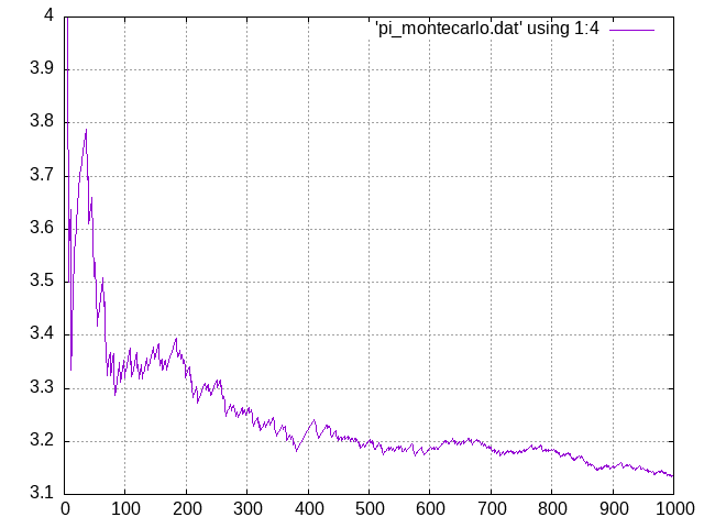
Figure 17.1.1 How the value of \(\pi\) improves with more darts used.

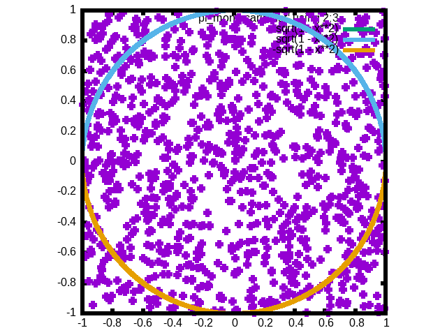
Figure 17.1.2 The places in which the darts landed.

To experiment further you can see what happens when you have as few as 100 darts, or as many as a million.

There are insights to be gained from both of these plots. The first plot shows you that the approximation to \(\pi\) is a painfully slow one. This is a general downside of monte carlo techniques: they are slow! You need huge numbers of darts before you start getting reasonable values for pi. Try adding many more darts to see how long it takes to get several digits of pi correctly.

The other insight comes from looking at the plot that shows the dart positions within the square. Notice how random numbers are not distributed evenly – that would be the opposite of random, since they would be more predicatble. The random generation of x and y gives us clusters and voides. This is why you need a lot of random numbers to calculate this area accurately.

17.1.2. Three dimensions: calculating the volume of a ball

The ideas from the 2-dimensional square-with-circle apply, but this time the program also generates a z coordinate, and we use the formula

\[V = \frac{4}{3} \pi r^3\]

Here is a download link to the program. You can then run it with:

chmod +x pi_montecarlo.dat
./ball_montecarlo.py > ball_montecarlo.dat
gnuplot
# then at the gnuplot> prompt you can type:
set grid
plot 'ball_montecarlo.dat' using 1:5 with lines
replot 'pi_montecarlo.dat' using 1:4 with lines

# in a separate terminal window you can run:
gnuplot
set view equal xyz
# then at the gnuplot> prompt you can type:
set samples 10000
set pm3d
splot [-1.1:1.1] [-1.1:1.1] [-1.1:1.1] 'ball_montecarlo.dat' using 2:3:4 with points pt 6 ps 0.5
replot [-1:1] sqrt(1 - x**2 - y**2) with pm3d
replot [-1:1] -sqrt(1 - x**2 - y**2) with pm3d

In these two examples (the disc and the ball) the analytic solution to the integral is not too difficult: one uses