1. Introduction and notes for teachers
test typesetting cross-references:
Introduction and notes for teachers
state of the book - 2025-10-06
At this time the “mostly-developed” working group is for the more advanced “math for research” in Part II -- Math for research: the chapter Approximating functions with series and the following chapters, aimed at upper grade high school students. These might also be interesting to students who have finished high school and never got that type of math. They might also be interesting to precocious middle school students who want to push ahead.
The more basic “visualizing algebra” part in Part I -- Visualizing algebra is coming together as a course starting with Chapter Introduction and notes for teachers: I have taught the working group twice, and have a clear idea of what is important for the students at that level. There is now an appendix with the detailed lesson plan I have used.
At this time “visualizing algebra” section that is best developed is Review of prerequisites. This has proven to be the most important chapter, and could maybe be split into a few chapters.
I also sometimes have a “physics with calculus” working groups, for which we use the OpenStax University Physics book [Ling, 2016]. Since we just work from that book, there is currently no section in this book for “physics with calculus”.
1.1. Overall motivation and plan
1.1.1. Visualizing algebra
The visualization of algebra is fun and mentally stimulating. This correspondence between algebra and geometry should be taught as a delightful romp: fun, amazing, and metaphorically rich.
It is also a key part of being able to attack a data set, understand it, and visualize it. The techniques used for that all make heavy use of this visualization of algebra.
Our plan is then to review how to visualize functions, and to show the details of it which make you fluent in understanding visualization of functions, data, and data analysis techniques.
This book will have very brief chapters and sections, deferring much of the specific work to the OpenSTAX book on Algebra and Trigonometry [Abramson, 2021]
A more complete motivation is given in the section Motivation and plan of the “Visualizing algebra” part of this book.
1.1.2. Math for research
Almost all math, including the math used in science and scholarship, does not have exact solutions. The quadratic formula, and the harmonic oscillator, are exceptions.
So in solving math problems we need to develop approximation techniques.
These techniques have been considered the domain of upper division college classes, but an effective computer user can get comfortable with many of these techniques a lot sooner.
The purpose of the math approximation working group is to use effective computer visualizations, and maybe a bit of programming, to learn some of the “numerical approximation” techniques.
We start by getting comfortable with visualization: we make sure that every student can use a plotting program, either on their computer (like gnuplot on linux systems) or GeoGebra or Desmos on the web.
And our practice of plotting gives us a review of polynomials, getting comfortable with how many extrema (max or min) and roots (zero crossings) a polynomial of \(n^{\rm th}\) degree has.
Then our real start consists of learning how to approximate transcendental functions (sin, cos, exp, …) with power series, and show how that can be applied to simplify the equation of the pendulum.
Then we will move on to Fourier analysis: the techniques to approximate functions with sums of sin and cosine functions.
After this we will look at how to approximate the calculation of areas: the field of numerical integration. We will also mention the whole world of monte carlo techniques for calculating integrals.
Then a discussion of how to solve differential equations that cannot be solved exactly.
More detailed motivation for, and a rambling introduction to, the “math for research” working group is in that part of the book: the sections Motivation for “math for research” and Rambling introduction.
1.2. Prerequisites
1.2.1. Visualizing algebra prerequisites
This working group has almost no prerequisites: basic algebra should be enough.
My experience is that many students in American schools take algebra, but then follow paths which allow them to not recall the details. This means that we will do a quick review of basic algebra, customized for the students in the working group.
1.2.2. Math for reseaerch prerequisites
The prerequisites vary according to who is in the working group: with a more advanced group of students we might assume that they know trigonometry, or even differential calculus.
The least we can assume is that the students should know something about polynomials. They might not know the name polynomial, but they should understand:
Visualizing them (this field is called analytic geometry): plotting a function of x versus x.
The equation for a straight line \(y = m x + b\)
The equation for a simple parabola \(y = x^2\). From here it is a simple matter to quickly introduce a diverse collection of parabolas, like \(y = -2x^2 - 3 x + 7\).
If some students have never seen those very simple polynomials then they can join the more fundamental math working group on visualizing algebra: Part I -- Visualizing algebra.
A good introduction to polynomials can be found in the openstax textbook on algebra and trigonometry. [Abramson, 2021]. To study from this book you can download the PDF file, or view it in a web browser. The chapter of interest is the one on polynomials and rational functions.
1.3. Notes for teachers
This book is not meant to be a text book for self study. It is meant to give an instructor examples for discussion and elaboration. Some of the text is also so that students can copy+paste instructions into a plotting program or web site.
The way I teach the course is driven by a few things:
The students are highly motivated.
They usually hear about the working groups because they have a diverse set of interests, and thus they see mathematics together with its links to other subjects. They also see math fitting in a historical tradition.
This is not something that they are required to do: they do it because they understand it’s important to go beyond school curriculum.
These selection effects mean that the students can work on material more advanced than their grade level.
1.4. A case to whet your appetite
There is a stark example of “being able to solve” versus “not being able to solve” as a problem acquires a bit of complexity: finding the roots of polynomials.
Remember that the roots of a polynomial \(y = p(x)\) are the values of \(x\) for which \(y = 0\).
1.4.1. Doing it graphically
Let’s say that you want to find all the places where the function
crosses the \(x\) axis. This is called finding the roots of the function.
Let us start by doing it graphically. Paste the following sequence into your plotting program:
1.2*x^2 - 4*x - 12
The plot tells you that the parabola has two zero crossings, approximately at “a bit more than -2” and one at “a bit more than 5”, as shown in Figure 1.4.1

Figure 1.4.1 Overall plot of the polynomial \(y = 1.2 x^2 - 4 x - 12\) - you can spot very rough values of the two roots.
If you zoom in on the left hand plot as shown in Figure 1.4.2 you can eventually resolve it to 3 digits of accuracy: somwhere between -1.9 and -1.91. You might even hazard the guess of approximately -1.908.
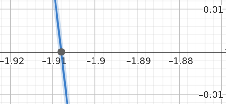
Figure 1.4.2 Same plot, but zooming in on the root to the left you can read off the approximate value of x for which \(y = 0\).
If you zoom in on the left hand plot as shown in Figure 1.4.3 you can eventually resolve it to 3 digits of accuracy: somwhere between 5.24 and 5.245. You might even hazard the guess of approximately 5.241.
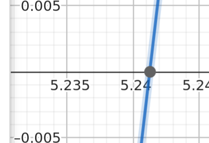
Figure 1.4.3 Same plot, but zooming in on the root to the right you can read off the approximate value of x for which \(y = 0\).
1.4.2. Quadratic formula
We have known for a long time how to calculate those solutions in closed form: using the general form for the second degree polynomial function \(y = a x^2 + b x + c\), the solution sare given by the quadratic formula
which in this case is:
This is much faster than the graphical approach we used.
So everything is fine, and we can calculate solutions to these problems. In math this is called a closed form solution, and when we find closed form solutions to problems we are very happy.
1.4.3. Let’s do a cubic graphically
Let us look at the third degree (“cubic”) polynomial:
How do we find its roots? Let us start with the graphical method. Paste this into your online plotting program:
x^3 + x^2 - 10*x - 2
and you find that there seem to be roots at around \((-3.7, -0.2, 2.8)\) and with a bunch of zooming you could find: \((-3.61, -0.197, 2.81)\).
This gets tiresome…
1.4.4. Cubic formula
So what about a formula for 3rd degree polynomials? Can you find its roots with a formula that might involve square roots or cube roots? The answer is yes: the polynomial function
has roots that can be written in closed form – a cubic formula.
The actual formula is so long that you will not see it written down in the same way as the quadratic formula – math books always introduce abbreviations to render it. The Wikipedia page on the cubic formula will give you many of the gory details, and this link on quora shows the full gory equation.
I show them here just to point out how they are not really useful:
and
and
Good luck making your browser window wide enough to see the full equations!
1.4.5. Quartic formula
So what about 4th degree polynomials? It turns out that, yes, there is a closed form solution. But this solution is even more complicated than the cubic, so we don’t see it written down often. Still, someone has posted it on quora, so here it is in its full majesty:
The 4 solutions to the polynomical equation
are given by:
1.4.6. Roots of higher order polynomials
We have learned two things:
Closed form solutions exist for 1st, 2nd, 3rd, and 4th degree polynomials. Polynomials and their solutions have a rich history - most of the low-order polynomials were known to ancient Babylonians (20th century BCE), who had tables to help calculate approximate solutions. Exact general algebraic solutions were discoved much later:
- quadratic - 9th century CE
General solution by al-Khwarizmi, the founder of Algebra.
- cubic - 16th century CE
General solution by Del Ferro and Tartaglia.
- quartic - 16th century CE
General solution by Ferrari.
They are not very useful beyond 2nd degree.
Now you might ask if closed form solutions exist for a fifth or higher degree polynomial. For a long time people sought out clever tricks, like those used for cubic and quartic, but it turned out to not be possible.
The general formulation of the question was:
Does there exist a formula for the roots of a fifth (or higher) degree polynomial equation in terms of the coefficients of the polynomial, using only the usual algebraic operations (addition, subtraction, multiplication, division) and application of radicals (square roots, cube roots, etc)?
After couple of centuries in which mathematicians hunted for these closed form solutions, French teenager Èvariste Galois developed a theory (Galois Theory) which allowed him to prove that polynomials of degree 5 or higher have no general closed form solutions.
Solutions obviously still exist for special cases, but there is nothing equivalent to the formulae shown above. They have to be calculated using a numerical algorithm.
This proof of the impossibility of finding a solution is one of the great achievements of mathematics, and it also means that we need to develop what are called numerical approximations to these problems, since we cannot write down exact expressions.
1.4.7. To conclude: how about symbolic algebra?
We will learn the rudiments of using the SymPy symbolic algebra system that runs inside Python. Since we have been looking at the roots of cubic polynomials, let us take a peek at how SymPy would find the roots of the one we looked at above:
To do this we can use the convenient web-based evaluator that the SymPy team offers. Go to the SymPy Gamma web site, and punch this into the text entry field:
roots(x**3 + x**2 - 10*x - 2)
You should get something like what is in Figure 1.4.4
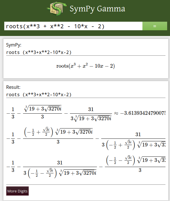
Figure 1.4.4 The roots of our cubic polynomial in closed form.
This is complicated and ugly (although exact); try to change from roots to real_roots:
real_roots(x**3 + x**2 - 10*x - 2)
and you will get the actual numbers as shown in Figure 1.4.5. Note that you easily get many more digits than with the graphical method, but they are close.
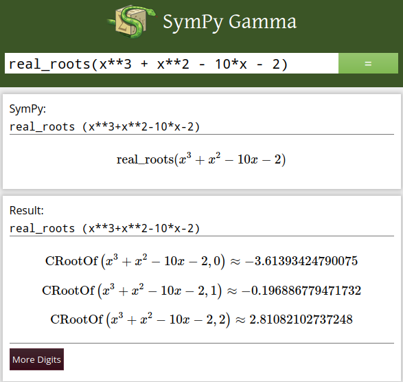
Figure 1.4.5 The roots of our cubic polynomial evaluated numerically. You see that the three roots are all real.
2. Logistics for specific courses
2.1. Winter/spring 2026 - math for research
First meeting:
Following meeting times:
Initial email:
Subject: math working group starts Feb. 2 - “Math for research”
Dear students,
TL;DR - Join us Monday, Feb. 2, 7pm US/Mountain (6pm US/Pacific, 8pm US/Central, 9pm US/Eastern) at https://meet.jit.si/math-working-group for the “Math for research” working group kick-off. Let me know if you want to be on the list. The material is described at https://markgalassi.codeberg.page/math-science-working-groups-html/math-for-research/motivation-and-review.html
Longer story:
From time to time we have a “math working group” where we explore areas of math that are crucial in preparing for advanced academic work and research.
Monday Feb. 2 2026 we will start the working group on “math for research”. The biggest focus is on the almost-daily techniques used by practicing scientists: approximating functions with Taylor series, Fourier analysis, solving differential equations numerically, and other topics. High schools do not teach these topics - some do a bit, but do not get far.
This is a no-anxiety working group. We get together and do serious work on advanced material, but you are always encouraged to say “hey, I did not get get that at all - can we step back?” You will find that everyone is happy when we slow down or step back! Also: if you ever feel that you are not as good as others, you’re wrong. Everyone steps in and out of doing well and being confused, and you will certainly be at both ends, even if you don’t notice. That’s what makes it OK to say “please, let’s step back”.
And most of the work we do will involve visualization to understand the advanced concepts, so at one level you can think of it as looking at pictures of math stuff and discussing the concepts :-)
We will meet on Monday evenings. If you cannot make it that’s OK: we will have a catch-up session on Wednesday evenings, and possibly another one on the weekend. The make-up is even more free-form where we can discuss any past material.
To see more detail on the material you can look at the book we will be using:
and the following chapters, starting with:
https://markgalassi.codeberg.page/math-science-working-groups-html/math-for-research/series.html
Finally: although this working group is fine as a free-standing course, it is also a key part of our pipline to prepare students for research, with a goal toward getting paid research internships. More information on the pipeline is at:
https://computinginresearch.org/our-pipeline-leading-students-to-research/
2.2. OLD: Fall/winter 2025 - visualizing algebra
First informational meeting:
First meeting:
Following meeting times:
Initial email to students:
subject-line: math working group starts Oct. 6 - “visualizing algebra”
Dear students,
TL;DR - Join us Monday, Oct. 6, 7pm US/Mountain time (6pm US/Pacific, 8pm US/Central, 9pm US/Eastern) at https://meet.jit.si/math-working-group for the “visualizing algebra” working group kick-off. Let me know if you want to join. The material is described at: https://markgalassi.codeberg.page/math-science-working-groups-html/visualizing-algebra/motivation-and-review.html
Longer story:
From time to time we have a “math working group” where we explore math differently from how it is done in school, adding elements that are crucial in preparing for advanced academic work and research.
Monday October 6 we will start “visualizing algebra” - the purpose is to build “agility and wide experience in visualizing equations and data”. We also do significant review of the algebra you learned a while ago, but we make it fun and memorable.
This is a no-anxiety working group. We get together and do real work, but you are always encouraged to say “hey, I did not get get that at all - can we step back?” You will find that everyone else is happy when we slow down or step back! Also: if you ever feel that you are not as good as others, you’re wrong. Everyone steps in and out of doing well and being confused, and you will certainly be at both ends, even if you don’t notice. That’s why it’s OK to say “please, let’s step back”.
And most of the work we do will involve visualization to understand the ideas, so at one level you can think of it as looking at pictures of math stuff and discussing the concepts :-)
We will meet on Monday evenings. If you cannot make it that’s OK: we will have a catch-up session on most Wednesday evenings, and on the weekend. The catch-up is even more free-form: in catch-up we can discuss any past material.
To see more detail on the material you can look at the “motivation and plan”: https://markgalassi.codeberg.page/math-science-working-groups-html/visualizing-algebra/motivation-and-review.html
Please reply to mark@galassi.org or call +1-505-629-0759 (voice only) if you are interested.
Kick-off meeting and first lesson:
At our initial meeting we will discuss various logistic matters, and get started doing math!
Expectations of students:
Students need to (a) do this for their own interest, not because of parental pressure; (b) manage their own correspondence entirely; (c) write from a non-school address; (d) Cc: a parent if the student is under 18 years old.
And…
If you cannot make the kick-off meeting, please write or call me and I will confirm the catch-up dates and times.
After this, in the depths of winter, we will kick off the more advanced “math for research” working group.
Initial email to teachers:
subject-line: math working group kick-off Monday Oct. 6 - “visualizing algebra”
Dear faculty,
[see attached flyer]
If you have students who are interested in math or advanced academic work of any kind please point them out way: we are kicking off this season’s math working groups. The first one that is about to start is also very good review for students with lacunae, or who have lingering “math blocks”.
The purpose is to give students some extra math tools which are useful when they work on research projects. This is part of the pipeline to prepare students for the Institute for Computing in Research, and internships beyond that.
The first one, “Visualizing algebra”, kicks off with an informational meeting and first lesson on Monday, October 6, 2025. This has plenty of review of basic algebra, along with material high school students do not see.
The more advanced one will start later in the winter: approximation techniques (Taylor series, Fourier series, numerical solutions to differential equations).
I hope you can point your students toward this working group. Overall info is at:
Students, or anyone interested, should email or call me and show up to the informational/kick-off meeting:
2.3. OLD: Winter/spring 2025 - math for research
First meeting:
Following meeting times:
Initial email:
Subject: math working group starts Feb. 3 - “Math for research”
Dear students,
TL;DR - Join us Monday, Feb. 3, 7pm US/Mountain (6pm US/Pacific, 8pm US/Central, 9pm US/Eastern) at https://meet.jit.si/math-working-group for the “Math for research” working group kick-off. Let me know if you want to be on the list. The material is described at https://markgalassi.codeberg.page/math-science-working-groups-html/math-for-research/motivation-and-review.html
Longer story:
From time to time we have a “math working group” where we explore areas of math that are crucial in preparing for advanced academic work and research.
Monday Feb. 3 2025 we will start the working group on “math for research”. The biggest focus is on the almost-daily techniques used by practicing scientists: approximating functions with Taylor series, Fourier analysis, solving differential equations numerically, and other topics. High schools do not teach these topics - some do a bit, but do not get far.
This is a no-anxiety working group. We get together and do serious work on advanced material, but you are always encouraged to say “hey, I did not get get that at all - can we step back?” You will find that everyone is happy when we slow down or step back! Also: if you ever feel that you are not as good as others, you’re wrong. Everyone steps in and out of doing well and being confused, and you will certainly be at both ends, even if you don’t notice. That’s what makes it OK to say “please, let’s step back”.
And most of the work we do will involve visualization to understand the advanced concepts, so at one level you can think of it as looking at pictures of math stuff and discussing the concepts :-)
We will meet on Monday evenings. If you cannot make it that’s OK: we will have a catch-up session on Wednesday evenings, and possibly another one on the weekend. The make-up is even more free-form where we can discuss any past material.
To see more detail on the material you can look at the book we will be using:
and the following chapters, starting with:
https://markgalassi.codeberg.page/math-science-working-groups-html/math-for-research/series.html
Finally: although this working group is fine as a free-standing course, it is also a key part of our pipline to prepare students for research, with a goal toward getting paid research internships. More information on the pipeline is at:
https://computinginresearch.org/our-pipeline-leading-students-to-research/
2.4. OLD: Fall/winter 2024 - visualizing algebra
First informational meeting:
First meeting:
Following meeting times:
Initial email to students:
subject-line: math working group starts Oct. 7 - “visualizing algebra”
Dear students,
TL;DR - Join us Monday, Oct. 7, 7pm US/Mountain time (6pm US/Pacific, 8pm US/Central, 9pm US/Eastern) at https://meet.jit.si/math-working-group for the “visualizing algebra” working group kick-off. Let me know if you want to join. The material is described at: https://markgalassi.codeberg.page/math-science-working-groups-html/visualizing-algebra/motivation-and-review.html
Longer story:
From time to time we have a “math working group” where we explore math differently from how it is done in school, adding elements that are crucial in preparing for advanced academic work and research.
Monday October 7 we will start “visualizing algebra” - the purpose is to build “agility and wide experience in visualizing equations and data”. We also do significant review of the algebra you learned a while ago, but we make it fun and memorable.
This is a no-anxiety working group. We get together and do real work, but you are always encouraged to say “hey, I did not get get that at all - can we step back?” You will find that everyone is happy when we slow down or step back! Also: if you ever feel that you are not as good as others, you’re wrong. Everyone steps in and out of doing well and being confused, and you will certainly be at both ends, even if you don’t notice. That’s why it OK to say “please, let’s step back”.
And most of the work we do will involve visualization to understand the ideas, so at one level you can think of it as looking at pictures of math stuff and discussing the concepts :-)
We will meet on Monday evenings. If you cannot make it that’s OK: we will have a catch-up session on most Wednesday evenings, and on the weekend. The catch-up is even more free-form: in catch-up we can discuss any past material.
To see more detail on the material you can look at the “motivation and plan”: https://markgalassi.codeberg.page/math-science-working-groups-html/visualizing-algebra/motivation-and-review.html
Please reply to mark@galassi.org or call +1-505-629-0759 (voice only) if you are interested.
Kick-off meeting and first lesson:
At our initial meeting we will discuss various logistic matters, and get started doing math!
Expectations of students:
Students need to (a) do this for their own interest, not because of parental pressure; (b) manage their own correspondence entirely; (c) write from a non-school address; (d) Cc: a parent if the student is under 18 years old.
And…
If you cannot make the kick-off meeting, please write or call me and I will confirm the catch-up dates and times.
After this, in the depths of winter, we will kick off the more advanced “math for research” working group.
Initial email to teachers:
subject-line: math working group kick-off Monday Oct. 7 - “visualizing algebra”
Dear faculty,
If you have students who are interested in math or advanced academic work of any kind, we are kicking off this season’s math working groups. The first one that is about to start is also very good review for students with lacunae, or who have lingering “math blocks”.
The purpose is to give students some extra math tools which are useful when they work on research projects. This is part of the pipeline to prepare students for the Institute for Computing in Research, and internships beyond that.
The first one, “Visualizing algebra”, kicks off with an informational meeting and first lesson on Monday, October 7, 2024. This has plenty of review of basic algebra, along with material high school students do not see.
The more advanced one will start later in the winter: approximation techniques (Taylor series, Fourier series, numerical solutions to differential equations).
I hope you can point your students toward this working group. Overall info is at:
Students, or anyone interested, should email or call me and show up to the informational/kick-off meeting:
2.5. OLD: Winter/spring 2024 - math for research
First meeting:
Following meeting times:
Initial email:
Subject: math working group starts Feb. 12 - “Math for research”
Dear students,
TL;DR - Join us Monday, Feb. 12, 8pm US/Mountain (7pm US/Pacific, 9pm US/Central, 10pm US/Eastern) at https://meet.jit.si/math-working-group for the “Math for research” working group kick-off. Let me know if you want to be on the list. The material is described at https://markgalassi.codeberg.page/math-science-working-groups-html/math-for-research/motivation-and-review.html
Longer story:
From time to time we have a “math working group” where we explore areas of math that are crucial in preparing for advanced academic work and research.
Monday Feb. 12 2024 we will start the working group on “math for research”. The biggest focus is on the almost-daily techniques used by practicing scientists: approximating functions with Taylor series, Fourier analysis, solving differential equations numerically, and other topics. High schools do not teach these topics - some do a bit, but do not get far.
This is a no-anxiety working group. We get together and do serious work on advanced material, but you are always encouraged to say “hey, I did not get get that at all - can we step back?” You will find that everyone is happy when we slow down or step back! Also: if you ever feel that you are not as good as others, you’re wrong. Everyone steps in and out of doing well and being confused, and you will certainly be at both ends, even if you don’t notice. That’s what makes it OK to say “please, let’s step back”.
And most of the work we do will involve visualization to understand the advanced concepts, so at one level you can think of it as looking at pictures of math stuff and discussing the concepts :-)
We will meet on Monday evenings. If you cannot make it that’s OK: we will have a catch-up session on Wednesday evenings, and possibly another one on the weekend. The make-up is even more free-form where we can discuss any past material.
To see more detail on the material you can look at the book we will be using:
and the following chapters, starting with:
https://markgalassi.codeberg.page/math-science-working-groups-html/math-for-research/series.html
2.6. OLD: Fall/winter 2023 - visualizing algebra
First informational meeting:
First meeting:
Following meeting times:
Initial email:
subject-line: math working group info/kick-off Monday October 30, 2023
Dear students and researchers,
In brief - math working groups to prepare for research are coming up: visualizing algebra now (Fall/Winter), and later we will have the advanced working group “math for research” in the winter. Please reply to mark@galassi.org or call +1-505-629-0759 (voice only) if you are interested.
Kick-off meeting:
date: Monday 2023-10-30 time: 8pm US/Mountain (7pm US/Pacific, 9pm US/Central, 10pm US/Eastern) location: https://meet.jit.si/math-working-group course name: visualizing algebra link to book: https://markgalassi.codeberg.page/math-science-working-groups-html/visualizing-algebra/motivation-and-review.html
At our informational meeting we will discuss (a) how often to meet (once or twice/week); (b) if we should meet at 8pm (US/Mountain time zone) or an hour later for our core meeting; (c) what days are best for catch-up sessions.
Then we will start the work!
More detail -
First of all: our format will be very flexible, with the opportunity for missing meetings - we will have make-up sessions, and frequent reviews of previous material.
Motivation:
The math we study in school often does not have the focus and examples that are important for real world research work. These working groups are an approach to solving this problem:
“””What do you do with real world problems, when textbook solutions do not work?”””
This first one, on visualizing algebra, is to build “agility and wide experience in visualizing equations and data.” It’s also to have fun with visualizations of cool functions.
Specific links:
motivation and plan: https://markgalassi.codeberg.page/math-science-working-groups-html/visualizing-algebra/motivation-and-review.html#motivation-and-plan
And…
If you cannot make the Monday October 30 kick-off meeting, please send your feedback on what times you can make.
After this, probably in the depths of winter, we will kick off the more advanced “math for research” working group.
2.7. OLD: Winter/spring 2023 - math for research
First meeting:
Following meeting times:
Initial email:
Subject: math working group starts Feb. 27 - “Math for research”
Dear students,
TL;DR - Join us Monday, Feb. 27, 8pm US/Mountain (7pm US/Pacific, 9pm US/Central, 10pm US/Eastern) at https://meet.jit.si/math-working-group for “Math for research” working group. Let me know if you want to be on the list.
Longer story:
Every now and then we have a “math working group” where we explore areas of math that are crucial in preparing for advanced academic work and research.
Monday Feb. 27 2023 we will start the working group on “math for research”. The biggest focus is on the almost-daily techniques used by practicing scientists: approximating functions with Taylor series, Fourier analysis, solving differential equations numerically, and other topics. High schools do not teach these topics - some do a bit, but do not get far.
This is a no-anxiety working group. We get together and do serious work on advanced material, but you are always encouraged to say “hey, I did not get get that at all - can we step back?” You will find that everyone is happy when we slow down or step back! Also: if you ever feel that you are not as good as others, you’re wrong. Everyone steps in and out of doing well and being confused, and you will certainly be at both ends, even if you don’t notice. That’s what makes it OK to say “please, let’s step back”.
And most of the work we do will involve visualization to understand the advanced concepts, so at one level you can think of it as looking at pictures of math stuff and discussing the concepts :-)
We will meet on Monday evenings. If you cannot make it that’s OK: we will have a catch-up session on Wednesday evenings, and possibly another one on the weekend. The make-up is even more free-form where we can discuss any past material.
To see more detail on the material you can look at the book we will be using:
and the following chapters, starting with:
https://markgalassi.codeberg.page/math-science-working-groups-html/math-for-research/series.html
2.8. OLD: Winter 2022-2023
2.8.1. (completed) visualizing algebra
This working group has been completed; the information is only here for archival purpose.
First meeting:
date: Monday 2022-12-01
time: 7pm US/Mountain (6pm US/Pacific, 8pm US/Central, 9pm US/Eastern)
location: https://meet.jit.si/math-working-group
Following meeting times:
New lessons: **Mondays** 8:00pm US/Mountain time (7:00pm US/Pacific,
9:00pm US/Central, 10:00pm US/Eastern)

Catch-up lessons: *Wednesdays* 8:00pm US/Mountain time and
*Saturdays* 10am US/Mountain time

location: https://meet.jit.si/math-working-group
Initial email:
Dear students and researchers,

In brief - math working groups to prepare for research are coming
up: visualizing algebra now, math approximations in
February.  Please reply to mark@galassi.org if you are interested.

Kick-off meeting:

date: Monday 2022-12-05
time: 7pm US/Mountain (6pm US/Pacific, 8pm US/Central, 9pm US/Eastern)
location: https://meet.jit.si/math-working-group
course name: visualizing algebra
link to book: https://markgalassi.codeberg.page/math-science-working-groups-html/

At our informational meeting we will discuss (a) how often to meet
(once or twice/week), (b) if we should meet at 7pm (US/Mountain
time zone) or an hour later.

Then we will start the work.

More detail -

First of all: our format will be very flexible, with the
opportunity for missing meetings - we will have make-up sessions,
and frequent reviews of previous material.

Motivation:

The math we study in school often does not have the focus and
examples that are important for real world research work.  These
working groups are an approach to solving this problem:

"""What do you do with real world problems, when textbook solutions
do not work?"""

This first one, on visualizing algebra, is to build "agility
and wide experience in visualizing equations and data."

Specific links:

motivation and plan:
https://markgalassi.codeberg.page/math-science-working-groups-html/visualizing-algebra/motivation-and-review.html

And...

If you cannot make the Monday December 5 kick-off meeting, please
send your feedback on what times you can make.

After this, probably in February, we will kick off the "math
approximations" working group.
2.8.2. Math approximations
Probably starting in February 2023.