In the previous chapter we learned about Fourier Analysis and showed
how to take the Fourier transform of some known functions.
Here we will show how to apply the Fourier transform to “data”, for
example to data coming from experiments. We will start with some
artificial data, and then look at the output from an experiment.
Until now we have discussed taking the Fourier transform of
a function: a signal \(s(t)\) that is either periodic or is
defined on a finite interval so that you can just duplicate it along
the \(t\) axis and make it become periodic.
But most of our applications will be with data, typically time
series data. At this point the instructor should discuss what
discrete data looks like.
This discussion of discrete data should not try to address every
possible issue — it is enough to show that you have the
correspondence of:
This might be the most universally used practical application of
Forier analysis, since it includes the subject of digital signal
processing, and hence the filtering of noisy data.
First a discussion of what noise is. The hiss of a tape, or
imperfections in an image (like blur) are examples. It is useful to
bring up an image of noise, and the Wikipedia article on white noise
has one:
At this point I zoom in on the waveform of Gaussian the white noise
signal to demonstrate what it looks like. I also play it on a speaker
so that the students can hear the hissing sound that is white noise.
If you add this noise to a meaningful signal then the signal might get
lost in the noise.
But Fourier analysis can come to the rescue: we can think of the
spectrum (how strong each frequency is in a signal) as a sort of
“character” of the signal, a deep description which might not be
obvious on the surface, but it is there.
Here we will do some experiments to demonstrate this idea, and then we
will use this idea to devise a marvel of data analysis: signal
filtering.
We start by building up some contrived signals and nibble around at
these contrived signals to get an intuition for how high frequency
\(sin()\) waves are suggestive of noise.
$ gnuplot
# at the gnuplot> prompt type:
set samples 1000
plot sin(x) + 0.3*sin(365*x)
and zoom in a lot. What initially looked like noise is now revealed
to be a high frequency sin wave added to the original.
Your zooming might suggest to you that the high frequency
\(\sin(365 x)\) term added spikes to the original signal. The
spikes were all the same height, so it is clearly not noise, but it is
suggestive of the fact that noise might come from high frequency
portions of the signal.
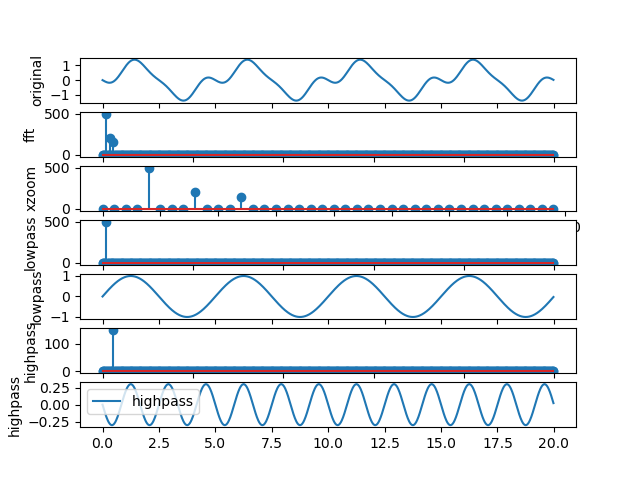
Now plot a simple superposition of three sin waves with period
\(T = 5\):
Figure 7.2.1 An example of filtering for a very simple signal: the sum of 3 sin
waves. The first filter zeros out all the high frequency fourier
coefficients (low pass filter). The second one zeroes out all the
low frequency fourier coefficients (high pass filter).
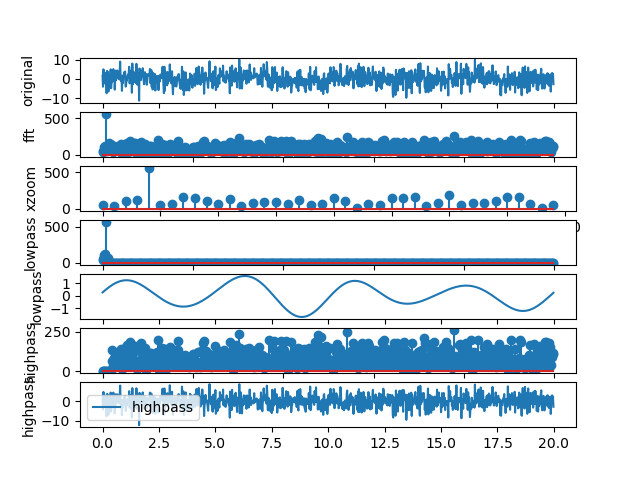
Figure 7.2.2 An example of filtering for a noisy signal: a sin() wave with
random noise added to it. The first filter zeros out all the high
frequency fourier coefficients (low pass filter). The second one
zeroes out all the low frequency fourier coefficients (high pass
filter).
The instructor can now experiment changing the
0.4*np.random.randn(...) to be 3.4* – this will dwarf the
signal with noise, but we will still find an approximate sin wave.
Another interest change is to apply the lowpass filter to the highpass
filter result (instead of to the original signal). This will give a
bandpass filter: a narrow band around the fundamental frequency.
Let us explore the data from a weather station. We will pick the Las
Cruces weather station from the climate research network coordinated
by NOAA (National Oceanic and Atmospheric Administration).
We will find that this data has both the features we saw above: it
has an underlying doubly periodic behavior, and it also has noise. It
also has plenty more information, related to weather (and, over the
course of many years) climate change, but we will focus on finding the
two periodic signals, and on the noise.
We spend a bit of time looking at the files “headers.txt” and
“readme.txt” to get a feeling for what the columns of data mean.
Once we know that column 4 (starting at 1) is local date, column 5 is
local time, and colum 9 is air temperature, we are ready to look at,
let’s say, the 2014 data for Las Cruces.
$ gnuplot
# then at the gnuplot> promt type:
plot 'CRNS0101-05-2014-NM_Las_Cruces_20_N.txt' using 9 with lines
We immediately see two undesirable spikes that come down to almost
-10000. We spend some time looking at the file, we puzzle over it,
and then realize that:
Caution
Data often needs cleaning. In this case you see that an old (and
poor) programmer habit crept into the pipeline of programs that
generated this data: when samples were missing they replaced them
with -9999.0.
We conclude that we have data spaced out by 5 minutes, and the 9th
column is a temperature reading, and that we need to eliminate all
lines that have -9999.0 in them. Remembering that grep-vexcludes all lines that match an expression, we can do:
$ grep-v9999CRNS0101-05-2014-NM_Las_Cruces_20_N.txt>Las_Cruces_filtered.txt
$ gnuplot
# thenatthegnuplot>prompttype:
plot 'Las_Cruces_filtered.txt' using 9 with lines
We might want to look at more than one year of data. We can do this
with:
for year in 2014 2015 2016
do
    wget --continue https://www.ncei.noaa.gov/pub/data/uscrn/products/subhourly01/${year}/CRNS0101-05-${year}-NM_Las_Cruces_20_N.txt
done
cat CRNS*Las_Cruces*.txt | grep -v -e -9999.0 > temperatures.dat
and now we have several years to plot:
$ gnuplot
$ # then at the gnuplot> prompt type:plot 'temperatures.dat' using 9 with lines
Now let us download the program code/temperature_fft.py
that analyzes this data with the fourier transform, and run it:
$ python3temperature_fft.py
Caution
These are big data files: 5 minute intervals for a year make for
more than 100 thousand samples per year. Three years of data will
require the Fourier transform of a signal with more than 300000
samples, which might strain the CPU and/or memory of your computer.
This might be even more of a problem if you use an web-based python
interpreter.
We have just gone through three examples of using the Fourier
transform on real data. This was a lot of new material, so let us
take a moment and discuss what we have seen.
First some terminology that accompanies these new ideas:
Continuous Fourier Transform
The coefficients of the sin and cos functions at various
frequencies which allow us to reproduce a periodic function of
continuous time. We discussed this in
Section 6
Discrete Fourier Transform (DFT)
A form of Fourier analysis that is applicable to a sequence of
values. Instead of a function \(f(t)\) with \(t\) being a
real number, we have a function given by pairs \({t_k, f_k}\).
The \(t_k\) values are discrete time samples, and \(f_k\)
are the samples of the function at those time points. The DFT is
clearly what we will be using to examine experimental data.
Fast Fourier Transform (FFT)
An algorithm to calculate the DFT in \(O(N\log N)\) time
instead of \(O(N^2)\). This is also known as the Cooley Tuckey
algorithm.
So is it DFT or FFT?
The FFT is used almost universally to calculate the DFT, so FFT is
sometimes used to mean the specific algorithm used, and sometimes
just as a placeholder for DFT.
Signal processing
A field of electrical engineering focused on analyzing, modifying,
and synthesizing signals. Signals can refer to sound, images, and
scientific measurements.
Noise
Unwanted distortions that a signal can suffer during propagation,
transmission, and processing. Often the specific origin of the
noise cannot be picked out, but it can be modeled in various ways
that help with finding a signal that might otherwise be obscured.
White noise
A form of noise that gets added to a signal and that has equal
intensity at different frequencies. In acoustics it sounds like a
hissing sound.