13. Fourier series: the “bones” of a function

There is often more to a plot than immediately meets the eye, and in the life of a scientist one of the great joys is to glean more information than what is on the surface.

Here we will show one of my favorite tools for extracting further information from data: the Fourier series. The result of this transformation is referred to as the Fourier spectrum of a signal.

Let us immediately dive in with a surprising example: breaking the square wave down into a sum of very round sin waves.

13.1. Fourier analysis: the square wave

Square waves are used as “clocks” in electronics: the edges can trigger logic circuits to do an action simultaneously with other circuits.

Figure 13.1.1 An example of timing diagram: the Synchronous Serial Peripheral Interface used for embedded system communication. Credit: Wikipedia

Let us start gnuplot and plot a \(\sin\) wave, then look at some \(\sin\) waves with higher frequencies. Then add them together and see what you get:

$ gnuplot
# and at the gnuplot> prompt:
set samples 1000
plot [] [-1.2:1.2] sgn(sin(x))
replot (4.0/pi) * sin(x)
replot (4.0/pi) * (1.0/3)*sin(3*x)
replot (4.0/pi) * (1.0/5)*sin(5*x)
replot (4.0/pi) * (sin(x) + (1.0/3)*sin(3*x) + (1.0/5)*sin(5*x))
## now look at the summed-up plot by itself:
plot (4.0/pi) * (sin(x) + (1.0/3)*sin(3*x) + (1.0/5)*sin(5*x)) t '5x'

In an online plotting calculator you might have:

sgn(sin(x))
(4/\pi) sin(x)
(4/\pi) (sin(x) + 1/3 sin(3 x))
(4/\pi) (sin(x) + 1/3 sin(3 x) + 1/5 sin(5 x))
(4/\pi) (sin(x) + 1/3 sin(3 x) + 1/5 sin(5 x) + 1/7 sin(7 x))
(4/\pi) (sin(x) + 1/3 sin(3 x) + 1/5 sin(5 x) + 1/7 sin(7 x) + 1/9 sin(9 x))
(4/\pi) (sin(x) + 1/3 sin(3 x) + 1/5 sin(5 x) + 1/7 sin(7 x) + 1/9 sin(9 x) + 1/11 sin(11 x))

You should start seeing that you go from a \(\sin\) wave to something that looks a bit more like a square wave. shows what the individual \(\sin\) waves look like and shows how you can add up to 13 of them and get something that starts to look quite square instead of wavy.

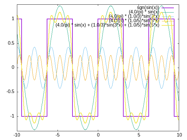
Figure 13.1.2 The first few terms of the Fourier series for the square wave.

This kind of series that sums up to the square function is called the Fourier series for the square wave. The full expression is:

\[s(t) = \frac{4}{\pi} \sum_{k=1}^{\infty} \frac{\sin((2k-1)\omega t)}{2k-1}\]

where \(\omega = 2\pi f\) is the angular frequency.

Note

Here the instructor should spend some time talking about the angular frequency. The nature of this conversation depends on how much exposure to physics the students have had. The simplest discussion of it could be that instead of counting how many times a periodic function repeats in a unit of time, we count how much angle a circular movement covers in a unit of time. Of course the angle is measured in radians, which is how we get \(\omega = 2\pi f\).

More generally you can approximate any periodic function with period \(T\) with the series:

\[s(t) = \sum_{k=0}^{\infty} \left( a_k\cos(k\omega t) + b_k\sin(k\omega t) \right)\]

where \(\omega = \frac{2\pi}{T}\).

Terminology:

fourier series

The way of writing a periodic function broken down as a sum of sin and cos waves with frequencies that are multiples of a fundamental frequency.

fourier coefficients

The values \(a_k \; {\rm and} \; b_k\) are the fourier coefficients for this function.

signal

One of the most active areas of science and engineering in which Fourier analysis is used is called signal processing, where we record electrical signals and analyze them in various ways. In this kind of setting we often use the word signal to mean the function we are discussing.

fourier spectrum

The ensemble of all of the fourier coefficients, \(\{a_k, b_k\}\), is called the fourier spectrum of the signal.

fourier transform

The technique that transforms a function of time into a function of frequency.

reciprocal space

The space in which the fourier coefficients live. For functions of time, the reciprocal space will be space of frequencies.

time domain and frequency domain

For signals that are a function of time, then the transform is a function of frequency. Both representations have the same information, so we sometimes talk about looking at the signal in the time domain or in the frequency domain.

13.2. Calculating the Fourier coefficients for periodic signals

We will talk here about periodic functions of a single real variable (we’ll call it \(t\)) with period \(T\). In these functions \(f(t + T) = f(t)\).

For this arbitrary periodic function \(f(t)\), the Fourier series for a signal \(s(t)\) with period \(\omega = \frac{2\pi}{T}\) is given by the expression shown above:

\[s(t) = \sum_{k=0}^{\infty} \left( A_k\cos(k\omega t) + B_k\sin(k\omega t) \right)\]

and the coefficients are given by:

\[\begin{split}A_k = \frac{2}{T} \int_0^T s(t) \cos(\frac{2\pi k}{T} t) dt \\ B_k = \frac{2}{T} \int_0^T s(t) \sin(\frac{2\pi k}{T} t) dt\end{split}\]

How do you derive these expressions for the \(a_n \; {\rm and} \; b_n\)? Start by remembering this fact from integration:

\[\begin{split}\int_0^{2\pi} \cos(m x) \cos(n x) dx = \begin{cases} \pi & \text{if} \; m = n \\ 0 & \text{if} \; m \ne n \end{cases}\end{split}\]

(Similar formulas apply to the \(\sin()\) function.)

This allows us to see that multiplying our series by \(\cos(m\omega t)\) will cause some simplifications when \(m \ne n\). We won’t look at the full derivation, which can be found as a straightforward result of searching for fourier series derivation - I just wanted to point out that this kind of integral over a full period of trigonometric functions allows us to pick out the coefficients.

Note

The fourier series is also sometimes written as:

\[s(t) = \sum_{k=1}^\infty D_k \cos\left( \frac{2\pi}{T} k t - \phi_k \right)\]

where the coefficients are \(D_k \; {\rm and} \; \phi_k\). The trigonometric identity for \(\cos(\alpha - \beta)\) will quickly show you that you can translate this into our sin + cos formula, mapping these coefficients to the \(A_k \; {\rm and} \; B_k\).

Caution

The Fourier transform is so often used in science, mathematics, engineering, and music that scholars have come up with many different conventions for how to write it. All these different conventions have slightly different notations or choices on whether to put certain factors in certain places, but they all end up having the same information. This means that when you read a paper where Fourier analysis is used, you have to look carefully to understand what convention they use. If the author did not specify a convention, then you should resent their sloppiness.

13.3. Developing intuition for the fourier coefficients

An expression like:

\[A_k = \frac{2}{T} \int_0^T s(t) \cos(\frac{2\pi k}{T} t) dt = \frac{2}{T} \int_0^T s(t) \cos(k \omega t) dt\]

can be daunting for a student: it has very many parts, and the instructor should spend some time breaking it down. What I do is to discuss all the letters that appear in the formula, preferring the second form that has \(\cos(k \omega t)\)

A_k

This is the coefficient that will multiply the \(\cos()\) term in the Fourier series. It has some analogy to the \(a_k\) term in the Taylor series \(f(x) = \sum_{k=0}^\infty a_k x^k\)

k

The \(k\) will be the integer multiple of the fundamental frequency. Remember… we’re talking about periodic signals \(s(t)\) which has angular frequence \(\omega = \frac{2\pi}{T}\)

T

The full period, which is related to \(\omega\) as I just showed. We integrate over a full period because the function is periodic, so all the information is contained in a full period.

t

The variable \(t\) inside the integral is just an integration variable - it does not appear outside. It will be used to step through the infinitely many little rectangles that form the integral.

\(k \omega t\)

I find this to be the most interesting thing to notice about the calculation of the transform: it is good to remember often that we are looking at trigonometric functions with integer multiples of a fundamental frequency \(\omega\). That fundamental frequence comes from the fact that the original signal is periodic.

After discussing those in detail, I often go to an online graphical calculator and have the students work with me at plotting a few periodic functions that are multiples of \(\sin()\) or \(\cos()\), and then of the square wave multiplies by \(sin()\).

This picture allows the students to see that the integral of the even terms over a period will always be zero, and that of the odd terms will not.

But maybe the best intuition will come from looking at the next section: a tour of some well-known periodic functions and their Fourier series.

13.4. A tour of functions and their Fourier series

We now apply our formulas for \(a_n \; {\rm and} \; b_n\) to a few common types of periodic signals. Remember that if it is periodic then we can just act like the function is defined on the interval \([0:2\pi]\) or \([-\pi:\pi]\). To get the full extent of the function we just duplicate that single period forever in both directions.

13.4.1. Sawtooth wave

\[f_{\rm sawtooth}(t) = \frac{1}{2} + \frac{t}{2} \; {\rm for} \; -1 < t \le 1\]

The coefficients are:

\[\begin{split}A_0 & = \; & \frac{1}{2} & \\ A_k & = & 0 & \;\;\;\;{\rm for}\; k \gt 0 \\ B_k & = & - \frac{1}{\pi} \frac{(-1)^k}{k} &\end{split}\]

So the series is:

\[f_{\rm sawtooth}(t) = \frac{1}{2} - \frac{1}{\pi} \sum_{k=1}^\infty \frac{(-1)^k}{k} \sin(k\pi t/T)\]

Let us plot this (using a period of \(T = 1\)) with:

reset
set grid
set samples 1000
set xrange [-2:2]
set yrange [-1.3:1.3]
# set terminal qt lw 2
plot 0 lw 1 lc 'black'
replot [-1:1] 1./2 + x/2 lw 2 lc 'green'
set arrow from -1, 0 to -1, 1 nohead lc 'green' lw 2
replot [1:2] 1./2 + x/2 - 1 lw 2 lc 'green'
set arrow from 1, 0 to 1, 1 nohead lc 'green' lw 2
replot [-2:-1] 1./2 + x/2 + 1 lw 2 lc 'green'
# that was the sawtooth wave.  pause to contemplate it, and then
# start with the Fourier series:
replot 1./2
replot 1./2 - 1/(pi)*( (-1)**1 * sin(1*pi*x)/1)
replot 1./2 - 1/(pi)*( (-1)**1 * sin(1*pi*x)/1 + (-1)**2 * sin(2*pi*x)/2)
replot 1./2 - 1/(pi)*( (-1)**1 * sin(1*pi*x)/1 + (-1)**2 * sin(2*pi*x)/2 + (-1)**3 * sin(3*pi*x)/3 + (-1)**4 * sin(4*pi*x)/4 + (-1)**5 * sin(5*pi*x)/5 + (-1)**6 * sin(6*pi*x)/6)
replot 1./2 - 1/(pi)*( (-1)**1 * sin(1*pi*x)/1 + (-1)**2 * sin(2*pi*x)/2 + (-1)**3 * sin(3*pi*x)/3 + (-1)**4 * sin(4*pi*x)/4 + (-1)**5 * sin(5*pi*x)/5 + (-1)**6 * sin(6*pi*x)/6 + (-1)**7 * sin(7*pi*x)/7 + (-1)**8 * sin(8*pi*x)/8 + (-1)**9 * sin(9*pi*x)/9 )
replot 1./2 - 1/(pi)*( (-1)**1 * sin(1*pi*x)/1 + (-1)**2 * sin(2*pi*x)/2 + (-1)**3 * sin(3*pi*x)/3 + (-1)**4 * sin(4*pi*x)/4 + (-1)**5 * sin(5*pi*x)/5 + (-1)**6 * sin(6*pi*x)/6 + (-1)**7 * sin(7*pi*x)/7 + (-1)**8 * sin(8*pi*x)/8 + (-1)**9 * sin(9*pi*x)/9 + (-1)**10 * sin(10*pi*x)/10 + (-1)**11 * sin(11*pi*x)/11 + (-1)**12 * sin(12*pi*x)/12 + (-1)**13 * sin(13*pi*x)/13 + (-1)**14 * sin(14*pi*x)/14 + (-1)**15 * sin(15*pi*x)/15 + (-1)**16 * sin(16*pi*x)/16 + (-1)**17 * sin(17*pi*x)/17 + (-1)**18 * sin(18*pi*x)/18 + (-1)**19 * sin(19*pi*x)/19 + (-1)**20 * sin(20*pi*x)/20 + (-1)**21 * sin(21*pi*x)/21 + (-1)**22 * sin(22*pi*x)/22 + (-1)**23 * sin(23*pi*x)/23 + (-1)**24 * sin(24*pi*x)/24 + (-1)**25 * sin(25*pi*x)/25 + (-1)**26 * sin(26*pi*x)/26 + (-1)**27 * sin(27*pi*x)/27 + (-1)**28 * sin(28*pi*x)/28 + (-1)**29 * sin(29*pi*x)/29 + (-1)**30 * sin(30*pi*x)/30 +  sin(31*pi*x)/31 )
# contemplate this for a moment and then let's simplify it by just
# plotting the last of those partial series:
reset
set samples 1000
plot 1./2 - 1/(pi)*( (-1)**1 * sin(1*pi*x)/1 + (-1)**2 * sin(2*pi*x)/2 + (-1)**3 * sin(3*pi*x)/3 + (-1)**4 * sin(4*pi*x)/4 + (-1)**5 * sin(5*pi*x)/5 + (-1)**6 * sin(6*pi*x)/6 + (-1)**7 * sin(7*pi*x)/7 + (-1)**8 * sin(8*pi*x)/8 + (-1)**9 * sin(9*pi*x)/9 + (-1)**10 * sin(10*pi*x)/10 + (-1)**11 * sin(11*pi*x)/11 + (-1)**12 * sin(12*pi*x)/12 + (-1)**13 * sin(13*pi*x)/13 + (-1)**14 * sin(14*pi*x)/14 + (-1)**15 * sin(15*pi*x)/15 + (-1)**16 * sin(16*pi*x)/16 + (-1)**17 * sin(17*pi*x)/17 + (-1)**18 * sin(18*pi*x)/18 + (-1)**19 * sin(19*pi*x)/19 + (-1)**20 * sin(20*pi*x)/20 + (-1)**21 * sin(21*pi*x)/21 + (-1)**22 * sin(22*pi*x)/22 + (-1)**23 * sin(23*pi*x)/23 + (-1)**24 * sin(24*pi*x)/24 + (-1)**25 * sin(25*pi*x)/25 + (-1)**26 * sin(26*pi*x)/26 + (-1)**27 * sin(27*pi*x)/27 + (-1)**28 * sin(28*pi*x)/28 + (-1)**29 * sin(29*pi*x)/29 + (-1)**30 * sin(30*pi*x)/30 +  sin(31*pi*x)/31 )

Users of geogebra can simply punch in:

1./2 - 1/(pi)*( (-1)**1 * sin(1*pi*x)/1 + (-1)**2 * sin(2*pi*x)/2 + (-1)**3 * sin(3*pi*x)/3 + (-1)**4 * sin(4*pi*x)/4 + (-1)**5 * sin(5*pi*x)/5 + (-1)**6 * sin(6*pi*x)/6 + (-1)**7 * sin(7*pi*x)/7 + (-1)**8 * sin(8*pi*x)/8 + (-1)**9 * sin(9*pi*x)/9 + (-1)**10 * sin(10*pi*x)/10 + (-1)**11 * sin(11*pi*x)/11 + (-1)**12 * sin(12*pi*x)/12 + (-1)**13 * sin(13*pi*x)/13 + (-1)**14 * sin(14*pi*x)/14 + (-1)**15 * sin(15*pi*x)/15 + (-1)**16 * sin(16*pi*x)/16 + (-1)**17 * sin(17*pi*x)/17 + (-1)**18 * sin(18*pi*x)/18 + (-1)**19 * sin(19*pi*x)/19 + (-1)**20 * sin(20*pi*x)/20 + (-1)**21 * sin(21*pi*x)/21 + (-1)**22 * sin(22*pi*x)/22 + (-1)**23 * sin(23*pi*x)/23 + (-1)**24 * sin(24*pi*x)/24 + (-1)**25 * sin(25*pi*x)/25 + (-1)**26 * sin(26*pi*x)/26 + (-1)**27 * sin(27*pi*x)/27 + (-1)**28 * sin(28*pi*x)/28 + (-1)**29 * sin(29*pi*x)/29 + (-1)**30 * sin(30*pi*x)/30 +  sin(31*pi*x)/31 )

As for Desmos, it has this problem where it does not handle a pasting-in of exponents with more than one digit. So you can punch in this expression where exponents are surrounded by {}. In addition \(\pi\) is written as \pi instead of pi to make the string pasting work for Desmos.

First put in the linear rising bit:

1 / 2 + x / 2

Then paste in a few terms of the sin approximation:

1./2 - 1/(\pi)*( (-1)^{1} * sin(1*\pi*x)/1 + (-1)^{2} * sin(2*\pi*x)/2)
1./2 - 1/(\pi)*( (-1)^{1} * sin(1*\pi*x)/1 + (-1)^{2} * sin(2*\pi*x)/2 + (-1)^{3} * sin(3*\pi*x)/3)
1./2 - 1/(\pi)*( (-1)^{1} * sin(1*\pi*x)/1 + (-1)^{2} * sin(2*\pi*x)/2 + (-1)^{3} * sin(3*\pi*x)/3 + (-1)^{4} * sin(4*\pi*x)/4)
1./2 - 1/(\pi)*( (-1)^{1} * sin(1*\pi*x)/1 + (-1)^{2} * sin(2*\pi*x)/2 + (-1)^{3} * sin(3*\pi*x)/3 + (-1)^{4} * sin(4*\pi*x)/4 + (-1)^{5} * sin(5*\pi*x)/5 + (-1)^{6} * sin(6*\pi*x)/6 + (-1)^{7} * sin(7*\pi*x)/7 + (-1)^{8} * sin(8*\pi*x)/8)
1./2 - 1/(\pi)*( (-1)^{1} * sin(1*\pi*x)/1 + (-1)^{2} * sin(2*\pi*x)/2 + (-1)^{3} * sin(3*\pi*x)/3 + (-1)^{4} * sin(4*\pi*x)/4 + (-1)^{5} * sin(5*\pi*x)/5 + (-1)^{6} * sin(6*\pi*x)/6 + (-1)^{7} * sin(7*\pi*x)/7 + (-1)^{8} * sin(8*\pi*x)/8 + (-1)^{9} * sin(9*\pi*x)/9 + (-1)^{10} * sin(10*\pi*x)/10 + (-1)^{11} * sin(11*\pi*x)/11 + (-1)^{12} * sin(12*\pi*x)/12)

Then paste in a lot of them:

1./2 - 1/(\pi)*( (-1)^{1} * sin(1*\pi*x)/1 + (-1)^{2} * sin(2*\pi*x)/2 + (-1)^{3} * sin(3*\pi*x)/3 + (-1)^{4} * sin(4*\pi*x)/4 + (-1)^{5} * sin(5*\pi*x)/5 + (-1)^{6} * sin(6*\pi*x)/6 + (-1)^{7} * sin(7*\pi*x)/7 + (-1)^{8} * sin(8*\pi*x)/8 + (-1)^{9} * sin(9*\pi*x)/9 + (-1)^{10} * sin(10*\pi*x)/10 + (-1)^{11} * sin(11*\pi*x)/11 + (-1)^{12} * sin(12*\pi*x)/12 + (-1)^{13} * sin(13*\pi*x)/13 + (-1)^{14} * sin(14*\pi*x)/14 + (-1)^{15} * sin(15*\pi*x)/15 + (-1)^{16} * sin(16*\pi*x)/16 + (-1)^{17} * sin(17*\pi*x)/17 + (-1)^{18} * sin(18*\pi*x)/18 + (-1)^{19} * sin(19*\pi*x)/19 + (-1)^{20} * sin(20*\pi*x)/20 + (-1)^{21} * sin(21*\pi*x)/21 + (-1)^{22} * sin(22*\pi*x)/22 + (-1)^{23} * sin(23*\pi*x)/23 + (-1)^{24} * sin(24*\pi*x)/24 + (-1)^{25} * sin(25*\pi*x)/25 + (-1)^{26} * sin(26*\pi*x)/26 + (-1)^{27} * sin(27*\pi*x)/27 + (-1)^{28} * sin(28*\pi*x)/28 + (-1)^{29} * sin(29*\pi*x)/29 + (-1)^{30} * sin(30*\pi*x)/30 +  sin(31*\pi*x)/31 )

(side note from Noah: Desmos tricks for sawtooth and triangle wave:)

Noah says:I accidentally did this last class cause I messed up the formula
Noah says:\frac{1}{2}\sum_{n=1}^{10}\frac{1}{n}\sin\left(n\pi x\right)
Noah
Noah says:\sum_{k=1}^{10}\frac{4(1-(-1)^{\left(2k-1\right)})}{\pi^{2}\left(2k-1\right)^{2}}\cos((2k-1)\pi x)
Noah says:second one is the even triangle

13.4.2. Triangle wave

Let us look at an even triangle wave. The Fourier series is:

\[f_{\rm EvenTriangle}(t) = \sum_{k=1}^\infty \frac{4(1 - (-1)^{k})}{\pi^2 (2k-1)^2} \cos((2k-1)\pi t)\]

$ gnuplot
# at the gnuplot> prompt type:
reset
set grid
set samples 1000
set xrange [-2:2]
set yrange [-1.3:1.3]
set terminal qt lw 2
plot 0 lw 1 lc 'black'
replot [-1:0] 2*x + 1 lw 2 lc 'green'
replot [1:2] 2*(x-1) - 1 lw 2 lc 'green'
replot [-2:-1] -2*x -3 lw 2 lc 'green'
replot [0:1] -2*x + 1 lw 2 lc 'green'
# now that we have a triangle wave, we try a few terms of the
# Fourier series
replot 4*(1 - (-1)**1)/(pi**2 * 1**2) * cos(1*pi*x)
replot 4*(1 - (-1)**1)/(pi**2 * 1**2) * cos(1*pi*x) + 4*(1 - (-1)**3)/(pi**2 * 3**2) * cos(3*pi*x)
replot 4*(1 - (-1)**1)/(pi**2 * 1**2) * cos(1*pi*x) + 4*(1 - (-1)**3)/(pi**2 * 3**2) * cos(3*pi*x) + 4*(1 - (-1)**5)/(pi**2 * 5**2) * cos(5*pi*x)
replot 4*(1 - (-1)**1)/(pi**2 * 1**2) * cos(1*pi*x) + 4*(1 - (-1)**3)/(pi**2 * 3**2) * cos(3*pi*x) + 4*(1 - (-1)**5)/(pi**2 * 5**2) * cos(5*pi*x) + 4*(1 - (-1)**7)/(pi**2 * 7**2) * cos(7*pi*x)
replot 4*(1 - (-1)**1)/(pi**2 * 1**2) * cos(1*pi*x) + 4*(1 - (-1)**3)/(pi**2 * 3**2) * cos(3*pi*x) + 4*(1 - (-1)**5)/(pi**2 * 5**2) * cos(5*pi*x) + 4*(1 - (-1)**7)/(pi**2 * 7**2) * cos(7*pi*x) + 4*(1 - (-1)**9)/(pi**2 * 9**2) * cos(9*pi*x)
# after contemplating each of those, put a *ton* of terms in there:
replot 4*(1 - (-1)**1)/(pi**2 * 1**2) * cos(1*pi*x) + 4*(1 - (-1)**3)/(pi**2 * 3**2) * cos(3*pi*x) + 4*(1 - (-1)**5)/(pi**2 * 5**2) * cos(5*pi*x) + 4*(1 - (-1)**7)/(pi**2 * 7**2) * cos(7*pi*x) + 4*(1 - (-1)**9)/(pi**2 * 9**2) * cos(9*pi*x) + 4*(1 - (-1)**11)/(pi**2 * 11**2) * cos(11*pi*x) + 4*(1 - (-1)**13)/(pi**2 * 13**2) * cos(13*pi*x) + 4*(1 - (-1)**15)/(pi**2 * 15**2) * cos(15*pi*x) + 4*(1 - (-1)**17)/(pi**2 * 17**2) * cos(17*pi*x) + 4*(1 - (-1)**19)/(pi**2 * 19**2) * cos(19*pi*x) + 4*(1 - (-1)**21)/(pi**2 * 21**2) * cos(21*pi*x) + 4*(1 - (-1)**23)/(pi**2 * 23**2) * cos(23*pi*x) + 4*(1 - (-1)**25)/(pi**2 * 25**2) * cos(25*pi*x) + 4*(1 - (-1)**27)/(pi**2 * 27**2) * cos(27*pi*x) + 4*(1 - (-1)**29)/(pi**2 * 29**2) * cos(29*pi*x) + 4*(1 - (-1)**31)/(pi**2 * 31**2) * cos(31*pi*x) + 4*(1 - (-1)**33)/(pi**2 * 33**2) * cos(33*pi*x) + 4*(1 - (-1)**35)/(pi**2 * 35**2) * cos(35*pi*x) + 4*(1 - (-1)**37)/(pi**2 * 37**2) * cos(37*pi*x) + 4*(1 - (-1)**39)/(pi**2 * 39**2) * cos(39*pi*x) + 4*(1 - (-1)**41)/(pi**2 * 41**2) * cos(41*pi*x) + 4*(1 - (-1)**43)/(pi**2 * 43**2) * cos(43*pi*x) + 4*(1 - (-1)**45)/(pi**2 * 45**2) * cos(45*pi*x) + 4*(1 - (-1)**47)/(pi**2 * 47**2) * cos(47*pi*x) + 4*(1 - (-1)**49)/(pi**2 * 49**2) * cos(49*pi*x) + 4*(1 - (-1)**51)/(pi**2 * 51**2) * cos(51*pi*x) + 4*(1 - (-1)**53)/(pi**2 * 53**2) * cos(53*pi*x) + 4*(1 - (-1)**55)/(pi**2 * 55**2) * cos(55*pi*x) + 4*(1 - (-1)**57)/(pi**2 * 57**2) * cos(57*pi*x) + 4*(1 - (-1)**59)/(pi**2 * 59**2) * cos(59*pi*x)

13.4.3. The Gaussian

The Fourier transform of a gaussian is fascinating from more than one point of view: the mathematical tricks used to calculate it are delightful and the applications are metaphorically rich.

13.4.3.1. Visuals on the Gaussian

Let us start by exploring the Gaussian function. We will use the form that gives the probability density function for a normally distributed random variable \(x\) with mean \(\mu\) and standard deviation \(\sigma\):

\[g(x) = \frac{1}{\sigma\sqrt{2\pi}} e^{-\frac{1}{2} \frac{(x - \mu)^2}{\sigma^2}}\]

If our mean is zero and standard deviation is one then we get:

\[g(x) = \frac{1}{\sqrt{2\pi}} e^{-x^2/2}\]

The Gaussian function comes up in so many places that it pays to become very comfortable with its behavior. Let us start with some plots to get a feeling for what it looks like:

reset
set grid
set terminal qt lw 3
set samples 1000
set xrange [-5:5]
set yrange [0:1]
plot (1.0/(1*sqrt(2*pi))) * exp(- (1./2) * (x - 0)**2 / 1**2) title 'mean 0 sigma 1'
replot (1.0/(2*sqrt(2*pi))) * exp(- (1./2) * (x - 0)**2 / 2**2) title 'mean 0 sigma 2'
replot (1.0/(0.5*sqrt(2*pi))) * exp(- (1./2) * (x - 0)**2 / 0.5**2) title 'mean 0 sigma 0.5'
replot (1.0/(0.4*sqrt(2*pi))) * exp(- (1./2) * (x - 1.3)**2 / 0.4**2) title 'mean 1.3 sigma 0.4'

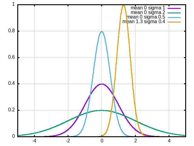
Figure 13.4.1 Gaussian curves for various standard deviations and a couple of means.

Looking closely at the formula for the Gaussian you will notice that \(\sigma\) appears in the denominator of the exponential, as well as the denominator of the constant scale factor \(\frac{1}{\sigma\sqrt{2\pi}}\). This means that:

\(\sigma\) is big

The curve will spread out and not be tall. This matches our intuition: if there is a big uncertainty then our random variable will often be quite different from the mean value.

\(\sigma\) is small

The curve will be skinny and taller. The intuition here is that random values are likely to be close to the mean, and not deviate from it much.

13.4.3.2. Normalization and total probability

If we think of the Gaussian as a probability distribution function then it is important that the probabilities of a random variable being in all its possible states add up to 1. This means that we insist that this integral:

\[\int_{-\infty}^{\infty} g(x) dx = \int_{-\infty}^{\infty} \frac{1}{\sigma\sqrt{2\pi}} e^{-\frac{1}{2} \frac{(x - \mu)^2}{\sigma^2}} dx\]

equal 1 for all values of \(\mu\) and \(\sigma\).

This is guaranteed by the Gaussian integral formula:

\[\int_{-\infty}^{\infty} e^{-x^2} dx = \sqrt{\pi}\]

If we substitute \(x \rightarrow ax\) then we get:

\[\begin{split}& \int_{-\infty}^{\infty} & e^{-a^2 x^2} d(ax) = a \int_{-\infty}^{\infty} e^{-a^2x^2} dx = \sqrt{\pi} \\ & \implies & \int_{-\infty}^{\infty} e^{-a^2x^2} dx = \sqrt{\pi} / a\end{split}\]

For the Gaussian our \(a^2\) is \(1 / (2\sigma^2)\), so we get:

\[\int_{-\infty}^{\infty} e^{-\frac{x^2}{2\sigma^2}} dx = \sqrt{\pi} / a = \sigma \sqrt{2\pi}\]

which implies that

\[\int_{-\infty}^{\infty} \frac{1}{\sigma \sqrt{2\pi}} e^{-\frac{x^2}{2\sigma^2}} dx = 1\]

This means that the Gaussian has been crafted carefully so that, no matter what \(\sigma\) is, we always end up with a total probability of 1.

The factor of \(\frac{1}{\sigma\sqrt{2\pi}}\) which multplies our exponential function is called a normalization constant. Normalization constants are widely used term in mathematics: we apply a constant scale to a function so that it satisfies some necessary condition.

Note that I have not mentioned the mean in discussing these integrals. The reason is that the gaussian goes from \(-\infty\) to \(\infty\), so a shift of the hump to the right or to the left does not affect the integral at all.

13.4.3.3. Fourier-transforming the Gaussian

The first thing I have to do here is be a bit apologetic: the Gaussian is not a periodic function. Nor is it defined on a finite domain (which can be treated as a periodic function. Rather, it unfolds on the entire real line with no repetitions.

This means that we cannot apply the mechanisms we saw earlier to calculate the Fourier transform of the Gaussian: this will be a different beast.

But the beast does exist: you can take an arbitrary function and write it down as a Fourier integral (not a sum; an integral!) which integrates sin and cos functions with a continuum of frequencies, and we will get our function back.

The Fourier transform of this more general function \(s(t)\) will not be a collection of discrete coefficients \({a_k}, {b_k}\) (remember: those \(k\) indices were multiples of a fundamental frequency).

Instead it will involve a pair of functions \(A(\omega), B(\omega)\) where \(\omega\) is the angular frequency \(\omega = 2 \pi f\):

\[s(t) = \int_{-\infty}^{\infty} \left( A(\omega) \cos(\omega t) + B(\omega) \sin(\omega t) \right) d\omega\]

You then calculate \(A(\omega)\) and \(B(\omega)\) quite analogously to the discrete Fourier coefficients:

\[\begin{split}A(\omega) = \frac{2}{\pi} \int_0^{\infty} s(t) \cos(\omega t) dt \\ B(\omega) = \frac{2}{\pi} \int_0^{\infty} s(t) \sin(\omega t) dt\end{split}\]

Let us apply this to the Gaussian. We will center it at a mean of zero then we have an even function. This means that \(B(\omega) = 0\), so we have: transform:

\[\begin{split}& g(t) & = \int_{-\infty}^{\infty} A(\omega) \cos(\omega t) d\omega \\ & {\rm where} & \\ & A(\omega) & = \frac{2}{\pi} \int_0^{\infty} g(t)cos(\omega t) dt = \frac{1}{\sigma\sqrt{2\pi}} \frac{1}{\pi} \int_{-\infty}^{\infty} e^{-t^2/(2\sigma^2)} \cos(\omega t) dt\end{split}\]

the application of some integration techniques gives us:

\[A(\omega) = \int_{-\infty}^{\infty} e^{-t^2/(2\sigma^2)} \cos(\omega t) dt = e^{-\sigma^2\omega^2/2}\]

The important thing to take home here is that the Fourier transform of a Gaussian is another Gaussian! And this other Gaussian has \(2/\sigma\) in all the places where the original one has \(\sigma\). If you let \(\delta = 2/\sigma\) then you get:

\[A(\omega) = e^{-\omega^2/(2\delta^2)}\]

so we can say that:

The Fourier transform of a Gaussian is a gaussian with the reciprocal standard deviation.

Caution

The equations above for \(s(t)\) and \(A(\omega)\) are subject to normalization. Researchers in different fields use a different normalization convention, with factors of 2 and \(\pi\) (possibly with square roots) that can be applied in one formula or in the other, as long as it is consistent. The lack of a single convention is frustrating, and ends up being costly, as collaborators have to be very careful. At this time I have not yet double-checked that I am using a uniform normalization convention in the equations above. Still, the fundamental conclusion holds: the transform of a Gaussian is a Gaussian with reciprocal standard deviation.

13.4.3.4. Visualization

Here is an animated visualization of the Gaussian and its transform for values of sigma that go from 10 to 1/10.

set grid
set samples 1000
do for [ii=1:100] {
    sigma = 10.0 / ii
     plot 1./(sigma*sqrt(2*pi)) * exp(-x**2 / (2*sigma**2))
     replot exp(-x**2 * sigma**2 / 4)
     pause(1.3)
}

We will show more visualizations when we look at uses of the Fourier transform on discrete data.

13.4.3.5. Thoughts about the transform of the Gaussian

[this section is not yet elaborated]

The general idea that if you have a narrowly localized signal in time, its Fourier transform will be spread out in frequency. Conversely, if you have a spread out signal, then its Fourier transform will be concentrated in a narrow band of frequencies.