2. Approximating functions with series

As I mentioned in the “motivation” section Section 1, apprimationg by series is a technique used almost daily by scientists. Let us dive in.

2.1. Sequences and sums

The classic definition of sequences and sums should be familiar.

For our purposes a sequence is an ordered list of numbers. We can index it with an integer. We can describe these sequences any way we want, for example in English we could say the sequence of all positive integers or the sequence of all positive odd numbers or even numbers and so forth.

Or we can describe them with examples of numbers where you can spot the pattern, or with math operations that map from integers to the numbers in our sequence. We often use curly braces to show that an index like \(i\) or \(k\) should be understood to cover all integers (or non-negative or positive integers). For example:

\[ \begin{align}\begin{aligned}\textrm{Natural numbers}: \{i\}: 1, 2, 3, 4, 5, \dots\\\textrm{Even numbers}: \{2i\}: 2, 4, 6, 8, 10, \dots\\\textrm{Odd numbers}: \{2i - 1\}: 1, 3, 5, 7, 9, \dots\end{aligned}\end{align} \]

The sum of a sequence is simply the addition of all numbers in that sequence. We use the classice uppercase \(\Sigma\) notation. For example:

\[\sum_{k=1}^{100} k = 1 + 2 + 3 + 4 + \dots + 100\]

In this notation the famous Gauss summation formula is:

\[\sum_{k=1}^{N} k = 1 + 2 + 3 + 4 + \dots + N = \frac{N (N+1)}{2}\]

An example of a function defined by a sum is the Riemann zeta function, defined as:

\[\zeta(s) = \sum_{k=1}^{\infty} \frac{1}{k^s}\]

We are not really going to study the Riemann zeta function here, but we are interested in one value, \(\zeta(2)\):

\[\zeta(2) = \sum_{k=1}^{\infty} \frac{1}{k^2} = \frac{\pi^2}{6}\]

This will give us an interesting playground to experiment with calculating values of \(\pi\).

Notice that a sum can be a finite sum or it can be a series: a sum of infinite terms where they get smaller and smaller so that the sum converges.

2.2. Do sums converge?

Convergence of series is a beautiful mathematical topic, but we will stick to our practical mode of operation here and mostly look at some examples to develop an intuition about it.

For example, the harmonic series diverges:

\[\sum_{k=1}^{\infty} \frac{1}{k}\]

which is interesting: it means that even though each number \(1/k\) is getting smaller and smaller, eventually tending to zero, the sum keeps growing without bounds.

Exercise: write a brief Python program which shows that if you pick any number, you can pick a number of terms of the harmonic series that gets bigger than that. Try it for a thousand, a million, then a billion, and see how many terms of the harmonic series you need to get bigger than that.

On the other hand, the alternating harmonic series:

\[\sum_{k=1}^{\infty} \frac{(-1)^{k+1}}{k} = 1 - \frac{1}{2} + \frac{1}{3} - \frac{1}{4} + \frac{1}{5} - \frac{1}{6} \dots = \log(2)\]

converges to the natural logarithm of 2. A variant of the alternating harmonic series with just the odd terms is called the Leibniz series:

\[\sum_{k=0}^{\infty} \frac{(-1)^k}{2k+1} = 1 - \frac{1}{3} + \frac{1}{5} - \frac{1}{7} + \frac{1}{9} \dots = \frac{\pi}{4}\]

2.3. Approximating pi with series

Calculate an approximation to \(\pi\) using the Leibniz series:

import math
sum = 0
N = 16
for i in range(0, N+1):
    term = (-1.0)**i / (2*i+1)
    sum += term
    pi_approx = 4.0 * sum
    print(i, '   ', term, '   ', sum, '   ', pi_approx)

And with the Riemann zeta function:

import math
sum = 0
N = 16
for i in range(1, N+1):
    term = 1.0 / (i*i)
    sum += term
    pi_approx = math.sqrt(6.0 * sum)
    print(i, '   ', term, '   ', sum, '   ', pi_approx)

2.4. A digression on the factorial

\[\begin{split}0! &= 1\\ 1! &= 1\\ 2! &= 2\times1\\ 3! &= 3\times2\times1 = 3\times2!\\ 4! &= 4\times3\times2\times1 = 4\times3!\\ 5! &= 5\times4\times3\times2\times1 = 5\times4!\\ \dots\\ n! &= n \times (n-1)!\end{split}\]

There is a function for real numbers called the gamma function which has the same value as the factorial (of one less) when it hits the nonnegative integers:

\[\Gamma(n) = (n-1)!\]

The full definition of the gamma function for all real (and in fact complex) numbers is more advanced. I show it here, but it is a subject for much later on:

\[\Gamma(z) = \int_0^\infty x^{z-1} e^{-x} dx\]

How fast does the factorial grow? Linear? Polynomial? Exponential? Something else?

We can study that question a bit with the following:

specific values

First in your head, then using a calculator, calculate 0!, 1!, 2!, 3!, …, 10!

the function

Then use the following plot commands to see the gamma function:

$ gnuplot
# then at the gnuplot> prompt:
set grid
set xrange [0:2]
plot gamma(1+x)    # this is equivalent to x! for integers
replot x**2
replot x**5
replot 2**x
replot exp(x)
# pause and examine
set xrange [0:3]
replot
# pause and examine
set xrange [0:4]
replot
# pause and examine
set xrange [0:5]
replot
# pause and examine
set xrange [0:6]
replot
# pause and examine
set xrange [0:7]
replot
# pause and examine
set xrange [0:8]
replot
# pause and examine
set xrange [0:9]
replot

Once you have tried to pit \(n!\) (or \(\Gamma(n+1)\)) against various exponential functions, take a look at Stirling’s approximation to the factorial:

\[n! \approx \sqrt{2\pi n}\left(\frac{n}{e}\right)^n\]

which is just the first term of a more elaborate series:

\[n! \approx \sqrt{2\pi n}\left(\frac{n}{e}\right)^n \left( 1 + \frac{1}{12 n} + \frac{1}{288 n^2} - \frac{139}{51840 n^3} - \frac{571}{2488320 n^4} + \dots \right)\]

Stirling’s formula is often used to calculate logarithms of \(n!\) like this:

\[\log n! = n \log n - n + O(\log n)\]

Looking closely at these formulae shows us that \(n!\) is indeed “super-exponential” in how it grows for large values of \(n\).

2.5. Experiments with series for sin and cos

We will start by doing experiments with the polynomials that give us approximations to \(\sin(x)\) and \(\cos(x)\).

2.5.1. Getting comfortable with radians

Remember: if a sensible angle feels like it’s in the range of 30 or 45 of 88 then it’s probably in degrees. If it’s expressed as \(\pi/4\), or some other multiple or fraction of \(\pi\), or a number that’s between 0 and 7, then there’s a good chance it’s measured in radians.

The conversion factor is \(\frac{\pi}{180}\) or its inverse \(\frac{180}{\pi}\):

\begin{eqnarray} \textrm{angle_radians} = \; & \textrm{angle_degrees} \times \frac{\pi}{180} \\ \textrm{angle_degrees} = \; & \textrm{angle_radians} \times \frac{180}{\pi} \end{eqnarray}

You should get comfortable with the everyday angles we use and what they are in radians: 90deg = pi/2, 60deg = pi/3, 45deg = pi/4, 30deg = pi/6.

A chart is at:

https://en.wikipedia.org/wiki/File:Degree-Radian_Conversion.svg

2.5.2. Making plots of polynomials that approximate sin and cos

Let us first generate plots that approximate sin and cos for very small angles:

\[ \begin{align}\begin{aligned}\sin(x) \approx x\\\cos(x) \approx 1\end{aligned}\end{align} \]

Use your favorite plotting program to show the following. I give the examples for gnuplot and for desmos and geogebra:

$ gnuplot
# then at the gnuplot> prompt:
set grid
plot [-1.5*pi:1.5*pi] [-1.5:1.5] sin(x)
replot x
replot cos(x)
replot 1

sin(x)
x
cos(x)
y = 1

Study this and make a guess as to where x is a good approximation to sin(x), and where 1 is a good approximation to cos(x). Set your calculator to radians and calculate how far off the approximation is for those values of x you come up with.

The next terms in the sin and cos series are:

\[ \begin{align}\begin{aligned}\sin(x) = x - \frac{x^3}{3!} + \frac{x^5}{5!} - \frac{x^7}{7!} + \frac{x^9}{9!} - \frac{x^{11}}{11!} \dots\\\cos(x) = 1 - \frac{x^2}{2!} + \frac{x^4}{4!} - \frac{x^6}{6!} + \frac{x^8}{8!} - \frac{x^{10}}{10!} \dots\end{aligned}\end{align} \]

Continue approximating the plots for sin and cos with higher degree polynomials, for example with the instructions below, and every time make an estimate (and then calculate it) for where they start diverging.

$ gnuplot
## then the following lines have the prompt gnuplot> and we type:
set grid
plot [-6:6] [-1.5:1.5] sin(x) lw 3
replot x
replot x - x**3 / 3!
replot x - x**3 / 3! + x**5 / 5!
replot x - x**3 / 3! + x**5 / 5! - x**7 / 7!
replot x - x**3 / 3! + x**5 / 5! - x**7 / 7! + x**9 / 9!

sin x
x
x - x^3 / 3!
x - x^3 / 3! + x^5 / 5!
x - x^3 / 3! + x^5 / 5! - x^7 / 7!
x - x^3 / 3! + x^5 / 5! - x^7 / 7! + x^9 / 9!

$ gnuplot
## then the following lines have the prompt gnuplot> and we type:
set grid
plot [-6:6] [-1.5:1.5] cos(x) lw 3
replot 1
replot 1 - x**2 / 2!
replot 1 - x**2 / 2! + x**4 / 4!
replot 1 - x**2 / 2! + x**4 / 4! - x**6 / 6!
replot 1 - x**2 / 2! + x**4 / 4! - x**6 / 6! + x**8 / 8!
replot 1 - x**2 / 2! + x**4 / 4! - x**6 / 6! + x**8 / 8! - x**10 / 10!

(cos x)
1
1 - x^2 / 2!
1 - x^2 / 2! + x^4 / 4!
1 - x^2 / 2! + x^4 / 4! - x^6 / 6!
1 - x^2 / 2! + x^4 / 4! - x^6 / 6! + x^8 / 8!
1 - x^2 / 2! + x^4 / 4! - x^6 / 6! + x^8 / 8! - x^10 / 10!

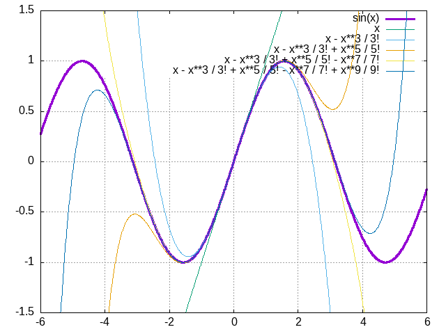
Figure 2.5.1 The first few polynomial approximations for the sin functions. The thicker line is the sin function, and the thinner ones are the ever-improving polynomial approximations.

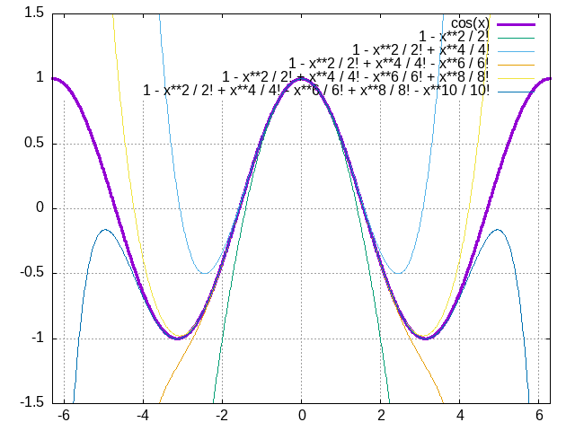
Figure 2.5.2 The first few polynomial approximations for the cos functions. The thicker line is the cos function, and the thinner ones are the ever-improving polynomial approximations.

What is the take-home from these two figures? What they show us is that you can approximate \(sin(x) \approx x\) for small values of \(x\). You can also approximate \(cos(x) \approx 1 - x^2/2!\) for small values of \(x\).